Demo 2：Gibbs 态制备

第 6 章 量子科学计算 · 本章演示 · 代码演示总索引

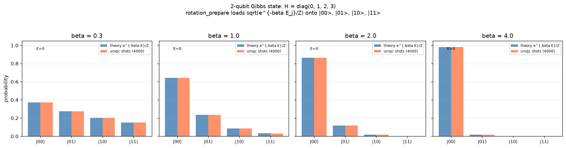
可视化：单子图（4 柱对比） —— 4 β 扫描的 P(|00⟩)=1/Z 反推

对应教程：第 6 章 量子科学计算 中相关小节 · 依赖安装：pip install "unified-quantum[visualization,simulation]"

实现要点

给定 H = diag(0, 1, 2, 3) 和逆温 beta，用 uniqc.rotation_prepare 直接将 Boltzmann 分布 |psi> = sum_j sqrt(e^{-beta E_j}/Z) |j> 装到 2 个 qubit 上。 扫描 beta 从低温到高温，展示不同温度下的概率分布与 H 矩阵本征结构。

完整源码

demos/ch06-scientific-computing/02_gibbs_state.py

"""
ch06 演示 2：2-qubit Gibbs 热态制备

对应教程：chenzhaoyun.com/quantum-tutorial/ch06-scientific-computing/gibbs-state.html
依赖：pip install unified-quantum[visualization]
运行：python demos/ch06-scientific-computing/02_gibbs_state.py

给定 H = diag(0, 1, 2, 3) 和逆温 beta，用 uniqc.rotation_prepare 直接将
Boltzmann 分布 |psi> = sum_j sqrt(e^{-beta E_j}/Z) |j> 装到 2 个 qubit 上。
扫描 beta 从低温到高温，展示不同温度下的概率分布与 H 矩阵本征结构。
"""
from __future__ import annotations

from pathlib import Path

import matplotlib
matplotlib.use("Agg")
import matplotlib.pyplot as plt
import numpy as np

from uniqc import Circuit, rotation_prepare, submit_task, wait_for_result

OUT = Path(__file__).parent

# --------------------------------------------------------------------------
# 1) 问题设定：H = diag(0, 1, 2, 3)，扫描 beta
# --------------------------------------------------------------------------
H_diag = np.array([0.0, 1.0, 2.0, 3.0])
betas = [0.3, 1.0, 2.0, 4.0]
n_shots = 4000

# 解析理论分布
def gibbs_probs(beta):
    weights = np.exp(-beta * H_diag)
    return weights / weights.sum()


# --------------------------------------------------------------------------
# 2) 对每个 beta 跑 uniqc，统计测量结果
# --------------------------------------------------------------------------
measured = {}
for beta in betas:
    target = np.sqrt(gibbs_probs(beta)).astype(complex)
    c = Circuit()
    rotation_prepare(c, target, qubits=[0, 1])
    c.measure(0)
    c.measure(1)
    task_id = submit_task(circuit=c, backend="dummy:local:simulator", shots=n_shots)
    result = wait_for_result(task_id)
    counts = result.counts
    total = sum(counts.values())
    measured[beta] = np.array([counts.get(bs, 0) / total
                               for bs in ("00", "01", "10", "11")])

# --------------------------------------------------------------------------
# 3) 可视化
# --------------------------------------------------------------------------
fig, axes = plt.subplots(1, len(betas), figsize=(4 * len(betas), 4.2),
                         sharey=True)

labels = [r"$|00\rangle$", r"$|01\rangle$", r"$|10\rangle$", r"$|11\rangle$"]
x_pos = np.arange(4)
w = 0.4

for ax, beta in zip(axes, betas):
    probs_th = gibbs_probs(beta)
    probs_emp = measured[beta]
    ax.bar(x_pos - w / 2, probs_th, w, label="theory e^{-beta E}/Z",
           color="steelblue", alpha=0.85)
    ax.bar(x_pos + w / 2, probs_emp, w,
           label=f"uniqc shots ({n_shots})", color="coral", alpha=0.85)
    ax.set_xticks(x_pos)
    ax.set_xticklabels(labels, fontsize=9)
    ax.set_title(f"beta = {beta}")
    ax.set_ylim(0, 1.05)
    ax.grid(True, alpha=0.3, axis="y")
    ax.legend(fontsize=7, loc="upper right")
    # annotate max
    j_max = int(np.argmax(probs_th))
    ax.text(j_max, 0.95, f"E={H_diag[j_max]:.0f}", ha="center", fontsize=8)

axes[0].set_ylabel("probability")

fig.suptitle("2-qubit Gibbs state: H = diag(0, 1, 2, 3)\n"
             "rotation_prepare loads sqrt(e^{-beta E_j}/Z) onto |00>, |01>, |10>, |11>",
             fontsize=11)
plt.tight_layout(rect=(0, 0, 1, 0.94))
plt.savefig(OUT / "02_gibbs_state.png", dpi=120, bbox_inches="tight")
plt.close()

# --------------------------------------------------------------------------
# 4) stdout 关键统计
# --------------------------------------------------------------------------
print("ch06-demo-2: 2-qubit Gibbs state via rotation_prepare")
print(f"  H eigenvalues (computational basis): {H_diag.tolist()}")
print(f"  shots per beta: {n_shots}")
for beta in betas:
    probs_th = gibbs_probs(beta)
    probs_emp = measured[beta]
    err = np.abs(probs_th - probs_emp).max()
    print(f"  beta={beta}: theory p00={probs_th[0]:.3f}, p01={probs_th[1]:.3f}, "
          f"p10={probs_th[2]:.3f}, p11={probs_th[3]:.3f}  max|err|={err:.4f}")

运行结果

运行方式

# 仓库根目录执行；输出 PNG 到 demos/ch06-scientific-computing/02_gibbs_state.png，关键统计到 stdout
.venv/bin/python3 demos/ch06-scientific-computing/02_gibbs_state.py

---

← 本章演示 · ↑ 代码演示总索引 · ⌂ 教程门户