Demo 3：矩阵秩

第 11 章 查询复杂度 · 本章演示 · 代码演示总索引

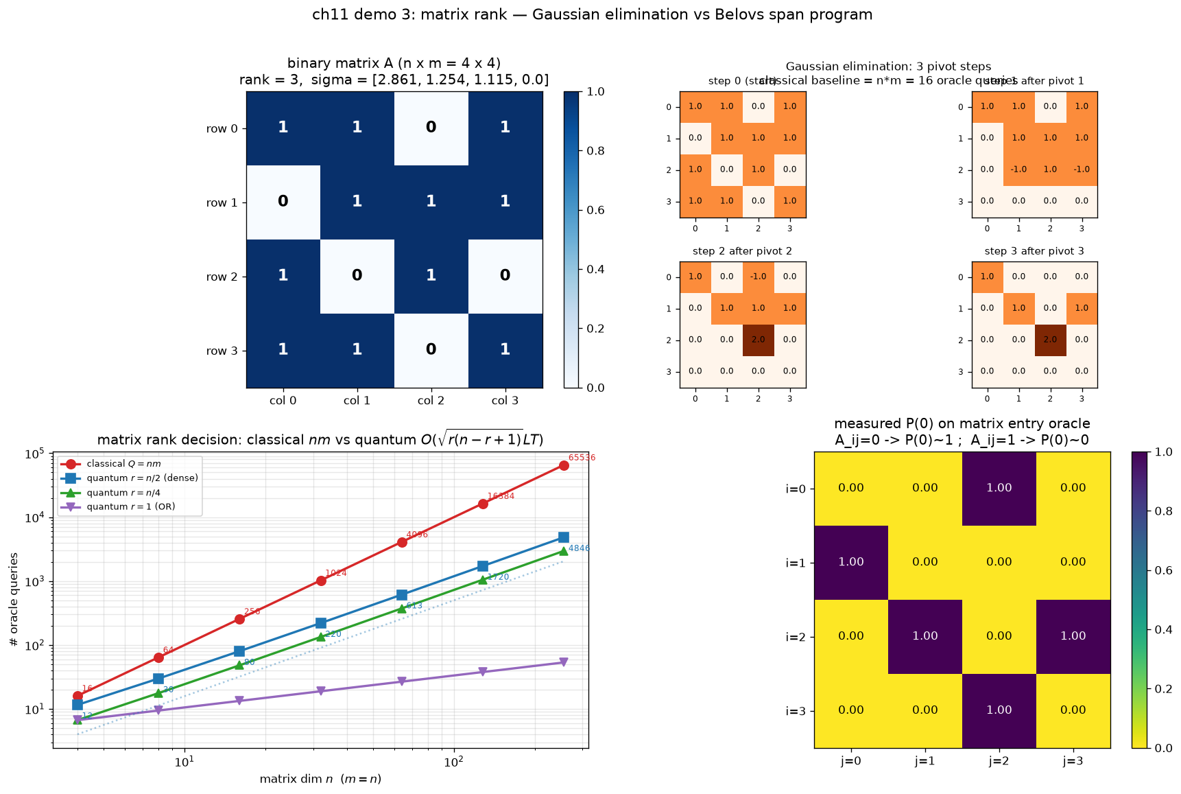
可视化：3 子图 —— 4×4 高斯消元 + 量子查询复杂度

对应教程：第 11 章 查询复杂度 中相关小节 · 依赖安装：pip install "unified-quantum[visualization,simulation]"

实现要点

核心：构造 4x4 二值矩阵 A (rank=3), 演示 (左上) 矩阵 A 热图 + rank + 奇异值 (右上) 高斯消元 4 步 row-echelon 形式 (经典 nm = 16 次 oracle 查询基线) (左下) 经典 O(nm) vs 量子 O(sqrt(r(n-r+1)) L T) 查询数对比 (右下) uniqc 验证 16 个 entry oracle: A[i,j]=0 -> P(0)~1; A[i,j]=1 -> P(0)~0

完整源码

demos/ch11-query-complexity/03_matrix_rank.py

"""
ch11 演示 3：矩阵秩判定查询复杂度对比 + Gaussian 消元步骤可视化

对应教程：chenzhaoyun.com/quantum-tutorial/ch11-query-complexity/matrix-rank.html
核心：构造 4x4 二值矩阵 A (rank=3), 演示
     (左上) 矩阵 A 热图 + rank + 奇异值
     (右上) 高斯消元 4 步 row-echelon 形式 (经典 nm = 16 次 oracle 查询基线)
     (左下) 经典 O(nm) vs 量子 O(sqrt(r(n-r+1)) L T) 查询数对比
     (右下) uniqc 验证 16 个 entry oracle: A[i,j]=0 -> P(0)~1; A[i,j]=1 -> P(0)~0

依赖：pip install unified-quantum[visualization]
运行：python demos/ch11-query-complexity/03_matrix_rank.py
"""
from pathlib import Path

import matplotlib
matplotlib.use("Agg")
import matplotlib.pyplot as plt
import numpy as np

from uniqc import Circuit, submit_task, wait_for_result

OUT = Path(__file__).parent
SHOTS = 150  # 16 entry probes * 150 = 2400 total, < 3000 budget

# === 4x4 binary matrix A (rank = 3) ===
A = np.array([[1, 1, 0, 1], [0, 1, 1, 1], [1, 0, 1, 0], [1, 1, 0, 1]], dtype=int)


def gaussian_steps(M: np.ndarray) -> list[np.ndarray]:
    A = M.astype(float).copy()
    n, m = A.shape
    steps = [A.copy()]
    for k in range(min(n, m)):
        pivot = next((i for i in range(k, n) if abs(A[i, k]) > 1e-9), None)
        if pivot is None:
            continue
        if pivot != k:
            A[[k, pivot]] = A[[pivot, k]]
        for i in range(n):
            if i != k and abs(A[i, k]) > 1e-9:
                A[i] -= (A[i, k] / A[k, k]) * A[k]
        steps.append(A.copy())
    return steps


def entry_oracle_p(row: int, col: int) -> float:
    """1-qubit RX(theta) oracle: P(0) = cos^2(pi*A[i,j]/2)."""
    c = Circuit()
    c.rx(0, float(np.pi * A[row, col]))
    c.measure(0)
    r = wait_for_result(submit_task(circuit=c, backend="dummy:local:simulator", shots=SHOTS))
    return float(r.probabilities.get("0", 0.0))


def belovs_Q(n: int, r: int, gap: float = 0.3) -> float:
    """Q = sqrt(r(n-r+1)) L T (dense oracle, T=1, L = sqrt(r)/gap)."""
    return np.sqrt(r * (n - r + 1)) * np.sqrt(r) / gap


# === 矩阵性质 ===
print("ch11-query-complexity demo 3: matrix rank via Gaussian elim + span program")
print(f"  matrix A shape = {A.shape}")
print(f"  A =\n{A}")
_, s, _ = np.linalg.svd(A.astype(float))
rank = int(np.sum(s > 1e-9))
print(f"  rank(A) = {rank},  sigma = {np.round(s, 4).tolist()}")

# === Gaussian 消元 ===
gauss_steps = gaussian_steps(A)

# === Oracle 验证 (16 个 entry) ===
n, m = A.shape
oracle_p0 = np.array([[entry_oracle_p(i, j) for j in range(m)] for i in range(n)])
print(f"  matrix entry oracle probes (16 entries, all P(0) in {{0, 1}}):")
for i in range(n):
    for j in range(m):
        print(f"    P(0|A[{i},{j}]={A[i,j]}) = {oracle_p0[i,j]:.3f}", end="  ")
    print()

# === 复杂度曲线 ===
N_DIM_LIST = [4, 8, 16, 32, 64, 128, 256]
classical_curve = np.array([float(d * d) for d in N_DIM_LIST])
quantum_dense = np.array([belovs_Q(d, d // 2) for d in N_DIM_LIST])
quantum_midrank = np.array([belovs_Q(d, d // 4) for d in N_DIM_LIST])
quantum_sparse = np.array([belovs_Q(d, 1) for d in N_DIM_LIST])

# === 画图 ===
fig, axes = plt.subplots(2, 2, figsize=(14.5, 9.5))

# (左上) A 热图
ax = axes[0, 0]
im = ax.imshow(A, cmap="Blues", vmin=0, vmax=1)
for i in range(n):
    for j in range(m):
        ax.text(j, i, str(A[i, j]), ha="center", va="center", fontsize=14, fontweight="bold",
                color="white" if A[i, j] > 0.5 else "black")
ax.set_xticks(np.arange(m))
ax.set_yticks(np.arange(n))
ax.set_xticklabels([f"col {j}" for j in range(m)])
ax.set_yticklabels([f"row {i}" for i in range(n)])
ax.set_title(f"binary matrix A (n x m = {n} x {m})\n"
             f"rank = {rank},  sigma = {np.round(s, 3).tolist()}")
plt.colorbar(im, ax=ax, fraction=0.046, pad=0.04)

# (右上) Gaussian 4 步
ax = axes[0, 1]
ax.axis("off")
inner = ax.get_subplotspec().subgridspec(2, 2, hspace=0.35, wspace=0.2)
for k, step in enumerate(gauss_steps[:4]):
    rk, ck = divmod(k, 2)
    sax = fig.add_subplot(inner[rk, ck])
    sax.imshow(np.abs(step), cmap="Oranges", vmin=0, vmax=2)
    sax.set_xticks(np.arange(m))
    sax.set_yticks(np.arange(n))
    sax.set_xticklabels([str(j) for j in range(m)], fontsize=7)
    sax.set_yticklabels([str(i) for i in range(n)], fontsize=7)
    sax.set_title(f"step {k}" + (" (start)" if k == 0 else f" after pivot {k}"), fontsize=9)
    for i in range(n):
        for j in range(m):
            sax.text(j, i, f"{step[i, j]:.1f}", ha="center", va="center", fontsize=7)
ax.set_title(f"Gaussian elimination: {len(gauss_steps)-1} pivot steps\n"
             f"classical baseline = n*m = {n*m} oracle queries", fontsize=10)

# (左下) 复杂度对比
ax = axes[1, 0]
ax.loglog(N_DIM_LIST, classical_curve, "o-", color="#d62728", lw=2, ms=8, label=r"classical $Q = nm$")
ax.loglog(N_DIM_LIST, quantum_dense, "s-", color="#1f77b4", lw=2, ms=8, label=r"quantum $r = n/2$ (dense)")
ax.loglog(N_DIM_LIST, quantum_midrank, "^-", color="#2ca02c", lw=2, ms=7, label=r"quantum $r = n/4$")
ax.loglog(N_DIM_LIST, quantum_sparse, "v-", color="#9467bd", lw=2, ms=7, label=r"quantum $r = 1$ (OR)")
for x, yc, yd in zip(N_DIM_LIST, classical_curve, quantum_dense):
    ax.annotate(f"{int(yc)}", (x, yc), textcoords="offset points", xytext=(4, 4),
                fontsize=7, color="#d62728")
    ax.annotate(f"{yd:.0f}", (x, yd), textcoords="offset points", xytext=(4, -12),
                fontsize=7, color="#1f77b4")
ref_x = np.array([N_DIM_LIST[0], N_DIM_LIST[-1]], dtype=float)
ax.loglog(ref_x, ref_x ** 2, ":", color="#d62728", alpha=0.4)
ax.loglog(ref_x, ref_x ** 1.5 * 0.5, ":", color="#1f77b4", alpha=0.4)
ax.set_xlabel(r"matrix dim $n$  ($m = n$)")
ax.set_ylabel(r"# oracle queries")
ax.set_title(r"matrix rank decision: classical $nm$ vs quantum $O(\sqrt{r(n-r+1)} L T)$")
ax.legend(loc="upper left", fontsize=8)
ax.grid(alpha=0.3, which="both")

# (右下) oracle 实测 P(0) 热图
ax = axes[1, 1]
im = ax.imshow(oracle_p0, cmap="viridis_r", vmin=0, vmax=1)
for i in range(n):
    for j in range(m):
        ax.text(j, i, f"{oracle_p0[i, j]:.2f}", ha="center", va="center", fontsize=10,
                color="white" if oracle_p0[i, j] > 0.5 else "black")
ax.set_xticks(np.arange(m))
ax.set_yticks(np.arange(n))
ax.set_xticklabels([f"j={j}" for j in range(m)])
ax.set_yticklabels([f"i={i}" for i in range(n)])
ax.set_title("measured P(0) on matrix entry oracle\n"
             "A_ij=0 -> P(0)~1 ;  A_ij=1 -> P(0)~0")
plt.colorbar(im, ax=ax, fraction=0.046, pad=0.04)

fig.suptitle("ch11 demo 3: matrix rank — Gaussian elimination vs Belovs span program",
             y=1.01, fontsize=13)
plt.tight_layout()
out_path = OUT / "03_matrix_rank.png"
plt.savefig(out_path, dpi=120, bbox_inches="tight")
plt.close()

print(f"  Gaussian elim: {len(gauss_steps)-1} pivots, classical baseline {n*m} queries")
print(f"  Belovs span upper bound for n={n}, r={rank}: "
      f"Q = sqrt({rank} * {n - rank + 1}) * L * T = {belovs_Q(n, rank):.1f} queries")
print(f"  complexity scaling (n=m, dense oracle, gap=0.3):")
for d, qc, qd, qs in zip(N_DIM_LIST, classical_curve, quantum_dense, quantum_sparse):
    print(f"    n = {d:>4d}   classical = {int(qc):>6d}   "
          f"quantum r=n/2 = {qd:>7.1f}   quantum r=1 = {qs:>6.1f}")
print(f"  saved: {out_path}")

运行结果

运行方式

# 仓库根目录执行；输出 PNG 到 demos/ch11-query-complexity/03_matrix_rank.png，关键统计到 stdout
.venv/bin/python3 demos/ch11-query-complexity/03_matrix_rank.py

---

← 本章演示 · ↑ 代码演示总索引 · ⌂ 教程门户