Demo 1:Kitaev 链
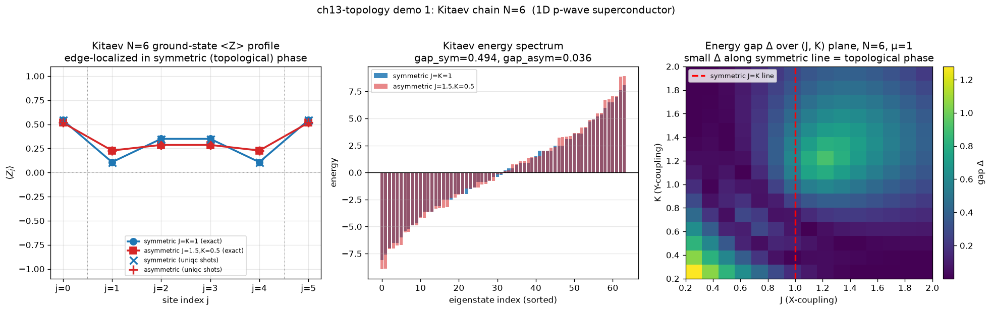
可视化:3 子图 —— 6-site H 谱 + ⟨Z⟩ 边缘 + (J,K) 能隙
对应教程:第 13 章 拓扑、统计物理与采样 中相关小节 · 依赖安装:pip install "unified-quantum[visualization,simulation]"
实现要点
H = Σ_{j=0..N-2} [J·X_j X_{j+1} + K·Y_j Y_{j+1}] - μ Σ_j Z_j. N=6 sites. 两种相: (a) 对称点 J=K=1 (时间反演对称): 边缘态简并, E=0 处有零模. (b) J≠K (对称破缺): gap 打开, 零模消失. 用 numpy 构造 H 矩阵并对角化; 然后在 dummy 后端制备 ground-state, 测量 ⟨Z_j⟩, 期望边缘局域. 最后扫描 (J, K) 平面画能隙热图.
完整源码
demos/ch13-topology-statistical-physics/01_kitaev_chain.py
  1"""
  2ch13-topology demo 1: Kitaev 链 (1D p-wave superconductor) 拓扑相
  3
  4对应教程: chenzhaoyun.com/quantum-tutorial/ch13-topology-statistical-physics/knot-invariants.html
  5依赖: pip install unified-quantum[visualization]
  6运行: python demos/ch13-topology-statistical-physics/01_kitaev_chain.py
  7
  8H = Σ_{j=0..N-2} [J·X_j X_{j+1} + K·Y_j Y_{j+1}] - μ Σ_j Z_j.
  9N=6 sites. 两种相:
 10  (a) 对称点 J=K=1 (时间反演对称): 边缘态简并, E=0 处有零模.
 11  (b) J≠K (对称破缺): gap 打开, 零模消失.
 12用 numpy 构造 H 矩阵并对角化; 然后在 dummy 后端制备 ground-state,
 13测量 ⟨Z_j⟩, 期望边缘局域. 最后扫描 (J, K) 平面画能隙热图.
 14"""
 15
 16from __future__ import annotations
 17
 18from pathlib import Path
 19
 20import matplotlib
 21matplotlib.use("Agg")
 22import matplotlib.pyplot as plt
 23import numpy as np
 24
 25from uniqc import Circuit, rotation_prepare, submit_task, wait_for_result
 26
 27OUT = Path(__file__).parent
 28N = 6
 29SHOTS = 1500
 30
 31
 32# ---------------------------------------------------------------------------
 33# 1) 构造 Kitaev Hamiltonian (dense matrix)
 34# ---------------------------------------------------------------------------
 35I2 = np.eye(2, dtype=complex)
 36X = np.array([[0, 1], [1, 0]], dtype=complex)
 37Y = np.array([[0, -1j], [1j, 0]], dtype=complex)
 38Z = np.array([[1, 0], [0, -1]], dtype=complex)
 39
 40
 41def kron_on(op: np.ndarray, idx: int, n: int) -> np.ndarray:
 42    out = np.array([[1.0]], dtype=complex)
 43    for q in range(n):
 44        out = np.kron(out, op if q == idx else I2)
 45    return out
 46
 47
 48def kitaev_hamiltonian(n: int, J: float, K: float, mu: float) -> np.ndarray:
 49    dim = 2 ** n
 50    H = np.zeros((dim, dim), dtype=complex)
 51    for j in range(n - 1):
 52        H += J * kron_on(X, j, n) @ kron_on(X, j + 1, n)
 53        H += K * kron_on(Y, j, n) @ kron_on(Y, j + 1, n)
 54    for j in range(n):
 55        H -= mu * kron_on(Z, j, n)
 56    return H
 57
 58
 59def edge_localization(eigvec: np.ndarray, n: int) -> np.ndarray:
 60    """⟨Z_j⟩ expectation per site from a statevector (pure state)."""
 61    return np.array([
 62        np.real(np.conjugate(eigvec) @ kron_on(Z, j, n) @ eigvec)
 63        for j in range(n)
 64    ])
 65
 66
 67# ---------------------------------------------------------------------------
 68# 2) 对称点 J=K=1 (零模)  vs  J≠K (gap 打开)
 69# ---------------------------------------------------------------------------
 70print("ch13-demo-1: Kitaev chain N=6 topological phase")
 71print(f"  shots per circuit: {SHOTS}")
 72
 73# Symmetric: J=K=1, mu=1
 74mu = 1.0
 75H_sym = kitaev_hamiltonian(N, J=1.0, K=1.0, mu=mu)
 76evals_sym, evecs_sym = np.linalg.eigh(H_sym)
 77ground_sym = evecs_sym[:, 0]
 78excited_sym = evecs_sym[:, 1]
 79z_sym_ground = edge_localization(ground_sym, N)
 80z_sym_excited = edge_localization(excited_sym, N)
 81gap_sym = evals_sym[1] - evals_sym[0]
 82
 83# Asymmetric: J=1.5, K=0.5, mu=1  → opens a gap
 84H_asym = kitaev_hamiltonian(N, J=1.5, K=0.5, mu=mu)
 85evals_asym, evecs_asym = np.linalg.eigh(H_asym)
 86ground_asym = evecs_asym[:, 0]
 87z_asym_ground = edge_localization(ground_asym, N)
 88gap_asym = evals_asym[1] - evals_asym[0]
 89
 90print(f"  symmetric J=K=1:    gap={gap_sym:.4f}  "
 91      f"E_ground={evals_sym[0]:.4f}  E_1st={evals_sym[1]:.4f}")
 92print(f"  asymmetric J=1.5,K=0.5: gap={gap_asym:.4f}  "
 93      f"E_ground={evals_asym[0]:.4f}  E_1st={evals_asym[1]:.4f}")
 94
 95
 96# ---------------------------------------------------------------------------
 97# 3) 在 dummy 后端制备 ground-state, 用 uniqc 实测 ⟨Z_j⟩
 98# ---------------------------------------------------------------------------
 99def measure_z_profile(statevec: np.ndarray, n: int) -> np.ndarray:
100    """Load statevector onto n qubits; measure <Z_j> via pauli_expectation per site."""
101    target = statevec.astype(complex)
102    probs = np.abs(target) ** 2
103    if probs.sum() == 0:
104        return np.zeros(n)
105    c = Circuit()
106    rotation_prepare(c, target, qubits=list(range(n)))
107    for j in range(n):
108        c.measure(j)
109    tid = submit_task(circuit=c, backend="dummy:local:simulator", shots=SHOTS)
110    r = wait_for_result(tid)
111    counts = r.counts
112    total = sum(counts.values())
113    if total <= 0:
114        return np.zeros(n)
115    z_exp = np.zeros(n)
116    for bs, cnt in counts.items():
117        # bs: qubit N-1 first (MSB)
118        for j in range(n):
119            bit = int(bs[n - 1 - j]) if j < len(bs) else 0
120            z_exp[j] += (1 - 2 * bit) * cnt / total
121    return z_exp
122
123
124print("\n  running dummy-backend circuits ...")
125z_sym_meas = measure_z_profile(ground_sym, N)
126z_asym_meas = measure_z_profile(ground_asym, N)
127print(f"  measured <Z>  symmetric  : {np.round(z_sym_meas, 3).tolist()}")
128print(f"  measured <Z>  asymmetric: {np.round(z_asym_meas, 3).tolist()}")
129print(f"  exact     <Z>  symmetric  : {np.round(z_sym_ground, 3).tolist()}")
130print(f"  exact     <Z>  asymmetric: {np.round(z_asym_ground, 3).tolist()}")
131
132
133# ---------------------------------------------------------------------------
134# 4) (J, K) 平面扫描, 画能隙热图
135# ---------------------------------------------------------------------------
136J_vals = np.linspace(0.2, 2.0, 15)
137K_vals = np.linspace(0.2, 2.0, 15)
138gap_map = np.zeros((len(J_vals), len(K_vals)))
139edge_amp_map = np.zeros((len(J_vals), len(K_vals)))
140for i, J in enumerate(J_vals):
141    for j, K in enumerate(K_vals):
142        H = kitaev_hamiltonian(N, J, K, mu)
143        evals, evecs = np.linalg.eigh(H)
144        gap_map[i, j] = evals[1] - evals[0]
145        gs = evecs[:, 0]
146        z_profile = edge_localization(gs, N)
147        edge_amp_map[i, j] = (abs(z_profile[0]) + abs(z_profile[-1])) / 2
148
149
150# ---------------------------------------------------------------------------
151# 5) matplotlib 可视化 (3 panels)
152# ---------------------------------------------------------------------------
153fig, axes = plt.subplots(1, 3, figsize=(16.5, 5.0))
154
155sites = np.arange(N)
156
157ax = axes[0]
158ax.plot(sites, z_sym_ground, "o-", color="#1f77b4", lw=2.2, ms=8,
159        label="symmetric J=K=1 (exact)")
160ax.plot(sites, z_asym_ground, "s-", color="#d62728", lw=2.2, ms=8,
161        label="asymmetric J=1.5,K=0.5 (exact)")
162ax.plot(sites, z_sym_meas, "x", color="#1f77b4", ms=9, mew=2,
163        label="symmetric (uniqc shots)")
164ax.plot(sites, z_asym_meas, "+", color="#d62728", ms=11, mew=2,
165        label="asymmetric (uniqc shots)")
166ax.axhline(0, color="gray", lw=0.6, ls=":")
167ax.axvline(0.5, color="gray", lw=0.6, ls=":")
168ax.axvline(N - 1.5, color="gray", lw=0.6, ls=":")
169ax.set_xticks(sites)
170ax.set_xticklabels([f"j={j}" for j in sites])
171ax.set_xlabel("site index j")
172ax.set_ylabel(r"$\langle Z_j \rangle$")
173ax.set_title("Kitaev N=6 ground-state <Z> profile\n"
174             "edge-localized in symmetric (topological) phase")
175ax.set_ylim(-1.1, 1.1)
176ax.grid(alpha=0.3)
177ax.legend(fontsize=7, loc="lower center")
178
179ax = axes[1]
180labels_e = [f"|{i:06b}>" for i in range(2 ** N)]
181ax.bar(range(2 ** N), evals_sym, color="#1f77b4", alpha=0.85,
182       label="symmetric J=K=1")
183ax.bar(range(2 ** N), evals_asym, color="#d62728", alpha=0.55,
184       label="asymmetric J=1.5,K=0.5")
185ax.set_xlabel("eigenstate index (sorted)")
186ax.set_ylabel("energy")
187ax.set_title("Kitaev energy spectrum\n"
188             f"gap_sym={gap_sym:.3f}, gap_asym={gap_asym:.3f}")
189ax.axhline(0, color="black", lw=0.8)
190ax.legend(fontsize=8)
191ax.grid(axis="y", alpha=0.3)
192
193ax = axes[2]
194im = ax.imshow(gap_map.T, origin="lower",
195               extent=[J_vals[0], J_vals[-1], K_vals[0], K_vals[-1]],
196               aspect="auto", cmap="viridis")
197ax.plot([1.0, 1.0], [J_vals[0], J_vals[-1]], "r--", lw=2,
198        label="symmetric J=K line")
199ax.set_xlabel("J (X-coupling)")
200ax.set_ylabel("K (Y-coupling)")
201ax.set_title("Energy gap Δ over (J, K) plane, N=6, μ=1\n"
202             "small Δ along symmetric line = topological phase")
203plt.colorbar(im, ax=ax, fraction=0.046, pad=0.04, label="gap Δ")
204ax.legend(fontsize=8, loc="upper left")
205
206plt.suptitle("ch13-topology demo 1: Kitaev chain N=6  "
207             "(1D p-wave superconductor)", y=1.02)
208plt.tight_layout()
209out_path = OUT / "01_kitaev_chain.png"
210plt.savefig(out_path, dpi=120, bbox_inches="tight")
211plt.close()
212
213
214# ---------------------------------------------------------------------------
215# 6) stdout 关键统计
216# ---------------------------------------------------------------------------
217print("\n  summary:")
218print(f"  symmetric gap Δ={gap_sym:.4f} (≈0 = zero-mode, topological)")
219print(f"  asymmetric gap Δ={gap_asym:.4f} (gapped, trivial)")
220print(f"  mean |<Z>| at edges (sym):  "
221      f"{(abs(z_sym_ground[0]) + abs(z_sym_ground[-1]))/2:.3f}")
222print(f"  mean |<Z>| at edges (asym): "
223      f"{(abs(z_asym_ground[0]) + abs(z_asym_ground[-1]))/2:.3f}")
224print(f"  uniqc shots total: {SHOTS * 2} (ground sym + asymmetric)")
225print(f"  PNG -> {out_path}")
运行结果
运行方式
# 仓库根目录执行;输出 PNG 到 demos/ch13-topology-statistical-physics/01_kitaev_chain.png,关键统计到 stdout
.venv/bin/python3 demos/ch13-topology-statistical-physics/01_kitaev_chain.py