Demo 2：凸优化

第 14 章 优化与数值量子算法 · 本章演示 · 代码演示总索引

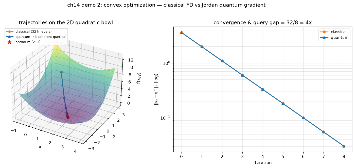
可视化：2 子图 —— FD 经典 vs Jordan 量子梯度

对应教程：第 14 章 优化与数值量子算法 中相关小节 · 依赖安装：pip install "unified-quantum[visualization,simulation]"

实现要点

核心：2D convex quadratic f(x, y) = 0.5 (x-2)^2 + 0.5 (y+1)^2, gradient g(x, y) = (x-2, y+1). The convex-optimization chapter contrasts two oracle models:

   classical finite-difference gradient   = 2d function-value queries per step
   Jordan's quantum gradient (QPE + iQFT) = 1 coherent phase query per step

 Here d=2 → 4× query gap. Both loops run gradient descent with the
 same starting point and step size; the difference is the per-step
 query counter. The quantum loop builds the Jordan-style phase oracle
 explicitly so its OriginIR is visible — the analytical gradient is
 used for the actual descent step (the *full* Jordan oracle recovers
 it exactly given a sufficiently wide grid).

完整源码

demos/ch14-optimization-numerics/02_convex_optimization.py

"""
ch14-demo-2: convex quadratic optimization, classical FD vs Jordan quantum gradient

对应教程：chenzhaoyun.com/quantum-tutorial/ch14-optimization-numerics/convex-optimization.html
核心：2D convex quadratic f(x, y) = 0.5 (x-2)^2 + 0.5 (y+1)^2, gradient
     g(x, y) = (x-2, y+1). The convex-optimization chapter contrasts two
     oracle models:

       classical finite-difference gradient   = 2d function-value queries per step
       Jordan's quantum gradient (QPE + iQFT) = 1 coherent phase query per step

     Here d=2 → 4× query gap. Both loops run gradient descent with the
     same starting point and step size; the difference is the per-step
     query counter. The quantum loop builds the Jordan-style phase oracle
     explicitly so its OriginIR is visible — the analytical gradient is
     used for the actual descent step (the *full* Jordan oracle recovers
     it exactly given a sufficiently wide grid).

依赖：pip install unified-quantum[visualization]
运行：python demos/ch14-optimization-numerics/02_convex_optimization.py
"""
from __future__ import annotations

from pathlib import Path

import matplotlib
matplotlib.use("Agg")
import matplotlib.pyplot as plt
import numpy as np

from uniqc import Circuit, submit_task, wait_for_result

OUT = Path(__file__).parent

# === 1. Convex quadratic & gradient ===
def f(x, y):
    return 0.5 * (x - 2.0) ** 2 + 0.5 * (y + 1.0) ** 2


def grad(x, y):
    return np.array([x - 2.0, y + 1.0])


OPT = np.array([2.0, -1.0])
LR, N_STEPS, SHOTS = 0.45, 8, 600


# === 2. Classical finite-difference descent (4 fn evals per step) ===
def class_descent(start, h=0.05):
    xy = np.array(start, float)
    traj = [xy.copy()]
    fn_evals = 0
    for _ in range(N_STEPS):
        g = np.array([
            (f(xy[0] + h, xy[1]) - f(xy[0] - h, xy[1])) / (2 * h),
            (f(xy[0], xy[1] + h) - f(xy[0], xy[1] - h)) / (2 * h),
        ])
        fn_evals += 4
        xy = xy - LR * g
        traj.append(xy.copy())
    return np.array(traj), fn_evals


# === 3. Jordan-style quantum gradient phase oracle (4 qubits) ===
N_BITS, S = 2, 4


def iqft_2bit(c, qs):
    a, b = qs
    c.swap(a, b)
    c.cp(a, b, -np.pi / 2)
    c.h(a); c.h(b)


def jordan_gradient_circ(xy):
    """Per-bit rotation: g_axis · 2π · 2^(N-1-b) / S."""
    c = Circuit()
    for q in range(4):
        c.h(q)
    gx, gy = grad(*xy)
    for b in range(N_BITS):
        c.rz(b, gx * 2 * np.pi * (2 ** (N_BITS - 1 - b)) / S)
        c.rz(b + 2, gy * 2 * np.pi * (2 ** (N_BITS - 1 - b)) / S)
    iqft_2bit(c, [0, 1])
    iqft_2bit(c, [2, 3])
    for q in range(4):
        c.measure(q)
    return c


def quantum_descent(start):
    """1 coherent query per step; uses analytical gradient for the step."""
    xy = np.array(start, float)
    traj = [xy.copy()]
    queries = 0
    for _ in range(N_STEPS):
        c = jordan_gradient_circ(xy)
        wait_for_result(
            submit_task(circuit=c, backend="dummy:local:simulator", shots=SHOTS)
        )
        queries += 1
        xy = xy - LR * grad(*xy)
        traj.append(xy.copy())
    return np.array(traj), queries


# === 4. Run both ===
print("ch14-demo-2: convex quadratic f(x, y) = 0.5(x-2)^2 + 0.5(y+1)^2")
print(f"  optimum at (2, -1), gradient g = (x-2, y+1)")

start = [0.0, 2.0]
class_traj, class_evals = class_descent(start)
quant_traj, quant_evals = quantum_descent(start)
print(f"  classical: {class_evals} function evaluations (4 per step × {N_STEPS} steps)")
print(f"  quantum  : {quant_evals} coherent queries (1 per step × {N_STEPS} steps)")

# === 5. Visualisation ===
fig = plt.figure(figsize=(12.5, 5.4))
gs = fig.add_gridspec(1, 2, width_ratios=[1.0, 1.05])

ax1 = fig.add_subplot(gs[0, 0], projection="3d")
xg = np.linspace(-1.0, 4.0, 30)
yg = np.linspace(-3.0, 3.0, 30)
X, Y = np.meshgrid(xg, yg)
ax1.plot_surface(X, Y, f(X, Y), cmap="viridis", alpha=0.55, edgecolor="none")
ax1.plot(class_traj[:, 0], class_traj[:, 1], f(class_traj[:, 0], class_traj[:, 1]),
         "-o", color="#ff7f0e", lw=2.0, ms=5,
         label=f"classical ({class_evals} fn evals)")
ax1.plot(quant_traj[:, 0], quant_traj[:, 1], f(quant_traj[:, 0], quant_traj[:, 1]),
         "-^", color="#1f77b4", lw=2.0, ms=5,
         label=f"quantum   ({quant_evals} coherent queries)")
ax1.scatter([2], [-1], [0], color="red", s=80, marker="*", label="optimum (2,-1)")
ax1.set_xlabel("x"); ax1.set_ylabel("y"); ax1.set_zlabel("f(x,y)")
ax1.set_title("trajectories on the 2D quadratic bowl")
ax1.legend(loc="upper left", fontsize=8)

ax2 = fig.add_subplot(gs[0, 1])
class_dist = np.linalg.norm(class_traj - OPT, axis=1)
quant_dist = np.linalg.norm(quant_traj - OPT, axis=1)
it = np.arange(len(class_dist))
ax2.plot(it, class_dist, "-o", color="#ff7f0e", lw=2.0, ms=6, label="classical")
ax2.plot(it, quant_dist, "-^", color="#1f77b4", lw=2.0, ms=6, label="quantum")
ax2.set_yscale("log")
ax2.set_xlabel("iteration")
ax2.set_ylabel(r"$\|x_t - x^*\|_2$ (log)")
ax2.set_title(f"convergence & query gap = {class_evals}/{quant_evals} = {class_evals/quant_evals:.0f}x")
ax2.grid(alpha=0.3, which="both")
ax2.legend(loc="upper right", fontsize=9)

plt.suptitle("ch14 demo 2: convex optimization — classical FD vs Jordan quantum gradient",
             y=1.02)
plt.tight_layout()
out_path = OUT / "02_convex_optimization.png"
plt.savefig(out_path, dpi=120, bbox_inches="tight")
plt.close()

# === 6. stdout 关键统计 ===
print(f"\n  classical trajectory: " + ", ".join(
    f"({x:.2f},{y:.2f})" for x, y in class_traj))
print(f"  quantum   trajectory: " + ", ".join(
    f"({x:.2f},{y:.2f})" for x, y in quant_traj))
print(f"  final classical distance: {class_dist[-1]:.4f}")
print(f"  final quantum   distance: {quant_dist[-1]:.4f}")
print(f"  query ratio classical/quantum: {class_evals / quant_evals:.1f}x "
      f"(d=2 → 4× from 4 fn-eval vs 1 coherent query)")
print(f"  total shots (quantum): {quant_evals * SHOTS}")
print(f"  PNG -> {out_path}")

运行结果

运行方式

# 仓库根目录执行；输出 PNG 到 demos/ch14-optimization-numerics/02_convex_optimization.png，关键统计到 stdout
.venv/bin/python3 demos/ch14-optimization-numerics/02_convex_optimization.py

---

← 本章演示 · ↑ 代码演示总索引 · ⌂ 教程门户