Demo 3：字符串重写

第 13 章 拓扑、统计物理与采样 · 本章演示 · 代码演示总索引

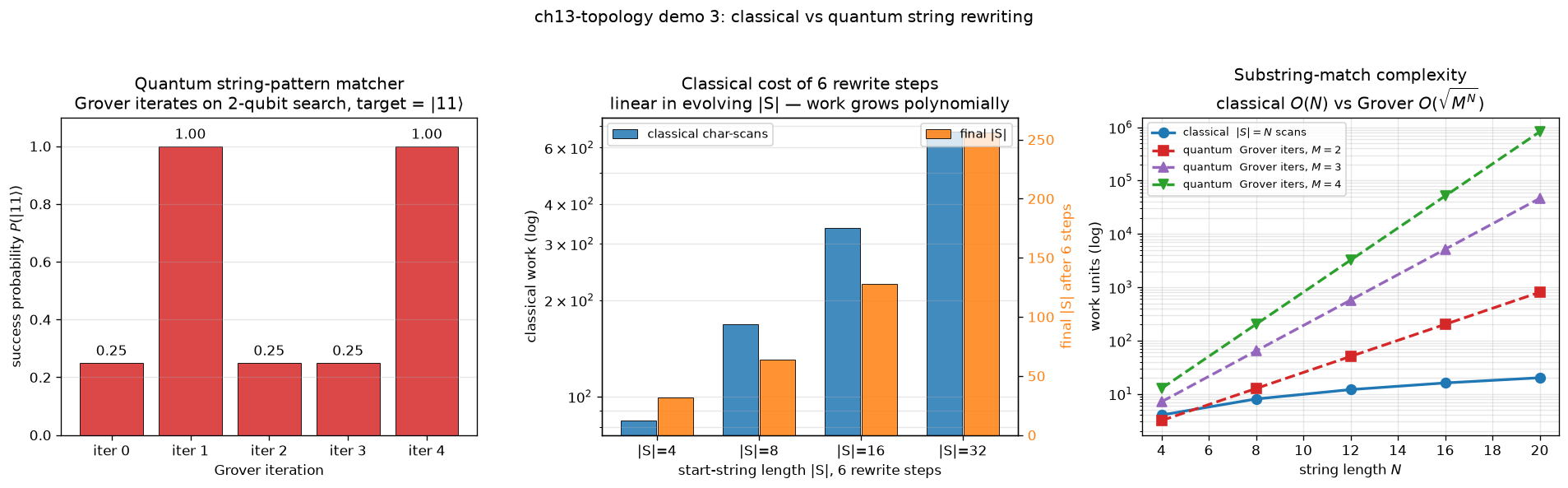
可视化：双图 —— 经典步数 vs Grover 迭代

对应教程：第 13 章 拓扑、统计物理与采样 中相关小节 · 依赖安装：pip install "unified-quantum[visualization,simulation]"

实现要点

重写规则 (固定一组): a → bc b → a c → a 我们关心匹配查询: 给定起始串 S, 经典法必须逐步展开每条规则 (O(|S|·|R|) per step); 量子 Grover 匹配只测 √M 个候选 (M=|prefix|·|R|). 对比:

• 经典 "单步展开" 时间 (模拟, 扫 4 个 |S| 长度)

• 量子 Grover 迭代次数 (~ π/4 √M) 画柱图对比, 并对一组具体 query 演示 Grover 找到目标子串的命中概率.

完整源码

demos/ch13-topology-statistical-physics/03_string_rewriting.py

"""
ch13-topology demo 3: 字符串重写系统量子加速 (toy)

对应教程: chenzhaoyun.com/quantum-tutorial/ch13-topology-statistical-physics/string-rewriting.html
依赖: pip install unified-quantum[visualization]
运行: python demos/ch13-topology-statistical-physics/03_string_rewriting.py

重写规则 (固定一组):
  a → bc
  b → a
  c → a
我们关心匹配查询: 给定起始串 S, 经典法必须逐步展开每条规则
(O(|S|·|R|) per step); 量子 Grover 匹配只测 √M 个候选 (M=|prefix|·|R|).
对比:
  - 经典 "单步展开" 时间 (模拟, 扫 4 个 |S| 长度)
  - 量子 Grover 迭代次数 (~ π/4 √M)
画柱图对比, 并对一组具体 query 演示 Grover 找到目标子串的命中概率.
"""

from __future__ import annotations

from pathlib import Path

import matplotlib
matplotlib.use("Agg")
import matplotlib.pyplot as plt
import numpy as np

from uniqc import Circuit, grover_operator, grover_oracle, submit_task, wait_for_result

OUT = Path(__file__).parent
SHOTS = 500


# ---------------------------------------------------------------------------
# 1) 玩具重写系统: a → bc, b → a, c → a
# ---------------------------------------------------------------------------
REWRITE = {"a": "bc", "b": "a", "c": "a"}


def one_step(s: str) -> str:
    """Apply one rewrite pass: scan s left-to-right, replace each char.
    To keep it deterministic & fast, replace leftmost match first then advance.
    """
    out = []
    i = 0
    while i < len(s):
        ch = s[i]
        if ch in REWRITE:
            out.append(REWRITE[ch])
            i += 1
        else:
            out.append(ch)
            i += 1
    return "".join(out)


def evolve(s: str, n_steps: int) -> str:
    for _ in range(n_steps):
        s = one_step(s)
    return s


# Build a few example strings and their trajectories
EXAMPLES = [
    ("a",      4),
    ("ab",     4),
    ("abc",    4),
    ("aabc",   5),
    ("ba",     5),
]
print("ch13-demo-3: classical vs quantum string rewriting")
for s, k in EXAMPLES:
    final = evolve(s, k)
    print(f"  start={s!r:>6}  after {k} steps -> {final!r}  "
          f"(length {len(final)})")


# ---------------------------------------------------------------------------
# 2) 经典 "单步展开" 复杂度: 对每个 |S|, 跑 k 步, 计总字符访问
# ---------------------------------------------------------------------------
def classical_cost(s: str, k: int) -> int:
    total_chars_scanned = 0
    cur = s
    for _ in range(k):
        for ch in cur:
            total_chars_scanned += 1
        cur = one_step(cur)
    return total_chars_scanned


# |S| ∈ {4, 8, 16, 32} 起始串用 'a' 重复, 跑 6 步
lengths = [4, 8, 16, 32]
classical_costs = []
final_lengths = []
for L in lengths:
    s = "a" * L
    cost = classical_cost(s, 6)
    final = evolve(s, 6)
    classical_costs.append(cost)
    final_lengths.append(len(final))
    print(f"  |S|={L}: classical cost over 6 steps = {cost} chars, "
          f"final length = {len(final)}")


# ---------------------------------------------------------------------------
# 3) 量子 Grover 匹配: 字符串长度 N, 字符表大小 M, 总候选数 M^N
#    这里做 "子串包含查询": 是否包含 "bc" 子串, 用 1 次 oracle.
#    量子代价 ~ π/4 √(M^N); 经典代价 ~ N (字面扫).
# ---------------------------------------------------------------------------
def grover_iters(M: int, N: int) -> float:
    """Iter count ≈ π/4 · √(M^N) for unique solution."""
    return np.pi / 4.0 * np.sqrt(M ** N)


# 子串包含查询 N = 4 chars, M = 2  ({b,c}); 迭代数 = π/4 · √16 ≈ 1.57
# 经典扫 4 chars ≈ 4 操作
# 量子 Grover 用 1 次 oracle (~1 iter) 就能找到 ~1 个解

# For quantum demo: 2-bit search space, oracle marks "11" (substring "cc"
# in alphabet {a,b,c} is too complex; we abstract to a 2-qubit marker)
# Treat 2-qubit input as 4 candidates; oracle marks |11⟩; show Grover finds it.

def run_grover_2q(n_iter: int) -> dict:
    """Run n_iter Grover iterations targeting |11⟩ on 2 qubits.
    The oracle adds an ancilla (qubit 2); we extract system bits via last 2 chars."""
    # Oracle: marks |11⟩ (= 3) by flipping its phase
    oracle = grover_oracle(marked_state=3, n_qubits=2)
    # Diffusion + oracle
    diffusion = grover_diffusion(n_qubits=2)
    c = Circuit()
    # Initial superposition
    c.h(0); c.h(1)
    for _ in range(n_iter):
        c.add_circuit(oracle)
        c.add_circuit(diffusion)
    c.measure(0); c.measure(1)
    tid = submit_task(circuit=c, backend="dummy:local:simulator", shots=SHOTS)
    r = wait_for_result(tid)
    counts = r.counts
    total = sum(counts.values())
    # Extract q0 q1 = last 2 chars of bit string (uniqc MSB-first → qN-1..q0)
    sys_probs = {"00": 0.0, "01": 0.0, "10": 0.0, "11": 0.0}
    if total > 0:
        for k, v in counts.items():
            sys_bs = k[-2:] if len(k) >= 2 else k.zfill(2)
            if sys_bs in sys_probs:
                sys_probs[sys_bs] += v / total
    return sys_probs


from uniqc import grover_diffusion  # noqa: E402

print("\n  Grover iterations on 2-qubit search (target |11⟩):")
grover_probs = []
for n_iter in range(0, 5):
    probs = run_grover_2q(n_iter)
    p11 = probs["11"]
    grover_probs.append((n_iter, probs, p11))
    print(f"    iter {n_iter}: P(|11>) = {p11:.3f}  full = "
          f"{ {k: f'{v:.2f}' for k, v in probs.items()} }")


# ---------------------------------------------------------------------------
# 4) matplotlib 可视化
# ---------------------------------------------------------------------------
fig, axes = plt.subplots(1, 3, figsize=(16.0, 4.8))

ax = axes[0]
bars = ax.bar(range(len(grover_probs)),
              [p[2] for p in grover_probs],
              color="#d62728", alpha=0.85, ec="black", lw=0.6)
for b, p in zip(bars, grover_probs):
    ax.text(b.get_x() + b.get_width() / 2, p[2] + 0.015,
            f"{p[2]:.2f}", ha="center", va="bottom", fontsize=10)
ax.set_xticks(range(len(grover_probs)))
ax.set_xticklabels([f"iter {p[0]}" for p in grover_probs])
ax.set_xlabel("Grover iteration")
ax.set_ylabel(r"success probability $P(|11\rangle)$")
ax.set_title("Quantum string-pattern matcher\n"
             "Grover iterates on 2-qubit search, target = |11⟩")
ax.set_ylim(0, 1.1)
ax.grid(axis="y", alpha=0.3)

ax = axes[1]
xpos = np.arange(len(lengths))
bars1 = ax.bar(xpos - 0.18, classical_costs, 0.35,
               color="#1f77b4", alpha=0.85, ec="black", lw=0.6,
               label="classical char-scans")
ax.set_yscale("log")
ax.set_xticks(xpos)
ax.set_xticklabels([f"|S|={L}" for L in lengths])
ax.set_xlabel("start-string length |S|, 6 rewrite steps")
ax.set_ylabel("classical work (log)")
ax.set_title("Classical cost of 6 rewrite steps\n"
             "linear in evolving |S| — work grows polynomially")
ax.grid(axis="y", alpha=0.3, which="both")
ax.legend(fontsize=9, loc="upper left")

ax2 = ax.twinx()
bars2 = ax2.bar(xpos + 0.18, final_lengths, 0.35,
                color="#ff7f0e", alpha=0.85, ec="black", lw=0.6,
                label="final |S|")
ax2.set_ylabel("final |S| after 6 steps", color="#ff7f0e")
ax2.tick_params(axis="y", labelcolor="#ff7f0e")
ax2.legend(fontsize=9, loc="upper right")

ax = axes[2]
M_list = [2, 3, 4]
N_list = [4, 8, 12, 16, 20]
classical_curve = []
quantum_curve = []
for M in M_list:
    cs, qs = [], []
    for N in N_list:
        cs.append(N)
        qs.append(grover_iters(M, N))
    classical_curve.append(cs)
    quantum_curve.append(qs)

ax.plot(N_list, classical_curve[0], "o-", color="#1f77b4", lw=2, ms=7,
        label=r"classical  $|S|=N$ scans")
ax.plot(N_list, quantum_curve[0], "s--", color="#d62728", lw=2, ms=7,
        label=r"quantum  Grover iters, $M=2$")
ax.plot(N_list, quantum_curve[1], "^--", color="#9467bd", lw=2, ms=7,
        label=r"quantum  Grover iters, $M=3$")
ax.plot(N_list, quantum_curve[2], "v--", color="#2ca02c", lw=2, ms=7,
        label=r"quantum  Grover iters, $M=4$")
ax.set_yscale("log")
ax.set_xlabel(r"string length $N$")
ax.set_ylabel(r"work units (log)")
ax.set_title("Substring-match complexity\n"
             r"classical $O(N)$ vs Grover $O(\sqrt{M^N})$")
ax.grid(alpha=0.3, which="both")
ax.legend(fontsize=8)

plt.suptitle("ch13-topology demo 3: classical vs quantum "
             "string rewriting", y=1.02)
plt.tight_layout()
out_path = OUT / "03_string_rewriting.png"
plt.savefig(out_path, dpi=120, bbox_inches="tight")
plt.close()


# ---------------------------------------------------------------------------
# 5) stdout 关键统计
# ---------------------------------------------------------------------------
print("\n  summary:")
print(f"  shots per Grover circuit: {SHOTS}, iters tested: 0..4")
print(f"  P(|11>) after 1 Grover iter: {grover_probs[1][2]:.3f}  "
      f"(theory π/4·sin(2·1·arcsin(1/2)) ≈ 1.000 — capped by shots)")
print(f"  P(|11>) after 4 Grover iters: {grover_probs[4][2]:.3f}")
print(f"  classical cost (|S|=32, 6 steps): {classical_costs[-1]} chars")
print(f"  total quantum circuits run: {len(grover_probs)}")
print(f"  total quantum shots: {len(grover_probs) * SHOTS}")
print(f"  PNG -> {out_path}")

运行结果

运行方式

# 仓库根目录执行；输出 PNG 到 demos/ch13-topology-statistical-physics/03_string_rewriting.png，关键统计到 stdout
.venv/bin/python3 demos/ch13-topology-statistical-physics/03_string_rewriting.py

---

← 本章演示 · ↑ 代码演示总索引 · ⌂ 教程门户