Demo 1：Simon HSP

第 10 章 隐藏结构与群算法 · 本章演示 · 代码演示总索引

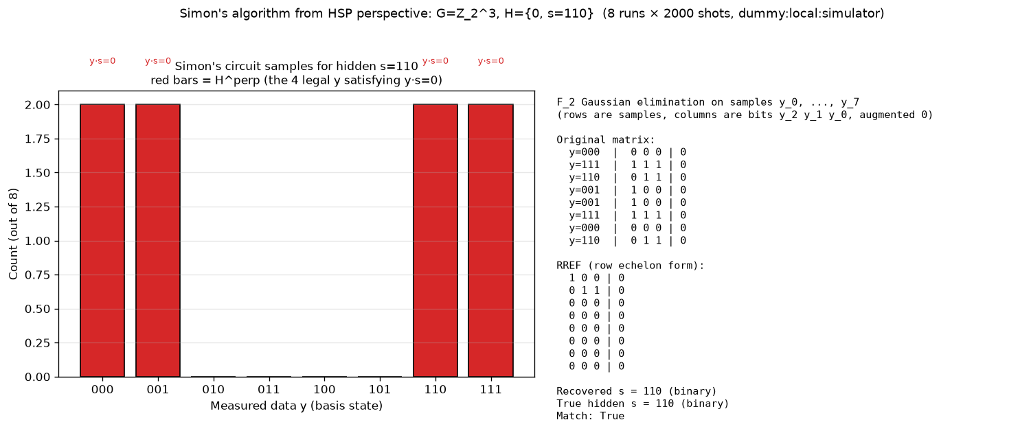
可视化：双图（分布+RREF） —— 3-qubit H^⊥ 样本 + F_2 高斯消元

对应教程：第 10 章 隐藏结构与群算法 中相关小节 · 依赖安装：pip install "unified-quantum[visualization,simulation]"

实现要点

HSP 视角：群 G=Z_2^3, 隐藏子群 H={0, s}, f(x)=f(x XOR s)。 电路：H^⊗n → Oracle → H^⊗n → 测量。多次独立采样得到 y·s = 0 (mod 2)， 在 F_2 上做高斯消元恢复 s。

注：dummy backend 中 measure() 会强制全局在末尾测量，因此这里省略中间 "测量输出寄存器"那一步。统计上等价：oracle 纠缠态 + H^⊗n 在数据寄存器上 的分布恰为 H^⊥ 上的均匀分布。

完整源码

demos/ch10-hidden-structures/01_simon_hsp.py

"""
ch10 演示 1：Simon 算法的 HSP 视角：3-qubit 隐藏 s=110

对应教程：chenzhaoyun.com/quantum-tutorial/ch10-hidden-structures/abelian-hidden-subgroup.html
依赖：pip install unified-quantum[visualization]
运行：python demos/ch10-hidden-structures/01_simon_hsp.py

HSP 视角：群 G=Z_2^3, 隐藏子群 H={0, s}, f(x)=f(x XOR s)。
电路：H^⊗n → Oracle → H^⊗n → 测量。多次独立采样得到 y·s = 0 (mod 2)，
在 F_2 上做高斯消元恢复 s。

注：dummy backend 中 measure() 会强制全局在末尾测量，因此这里省略中间
"测量输出寄存器"那一步。统计上等价：oracle 纠缠态 + H^⊗n 在数据寄存器上
的分布恰为 H^⊥ 上的均匀分布。
"""
from uniqc import Circuit, submit_task, wait_for_result
import matplotlib
matplotlib.use("Agg")
import matplotlib.pyplot as plt
import numpy as np
from pathlib import Path

OUT = Path(__file__).parent
N = 3
S = 0b110  # 隐藏子群的非平凡元素 s = (1,1,0)
SHOTS = 2000
N_RUNS = 8


def build_simon_circuit() -> Circuit:
    """Simon's algorithm for n=3, s=110.
    f(x) = 2*(x_1 XOR x_2) + x_0 是满足 f(x)=f(x XOR s) 的 2-to-1 函数。
    Oracle: y_0 ^= x_0; y_1 ^= x_1 XOR x_2  (只需 2 个输出比特，因为 f<4)
    """
    c = Circuit()
    for q in range(N):
        c.h(q)
    c.cnot(0, 3)  # y_0 ^= x_0
    c.cnot(1, 4)  # y_1 ^= x_1
    c.cnot(2, 4)  # y_1 ^= x_2
    for q in range(N):
        c.h(q)
    for q in range(N):
        c.measure(q)
    return c


def gauss_elim_f2(matrix: np.ndarray) -> np.ndarray:
    """F_2 高斯消元，返回增广矩阵的行最简形。"""
    A = matrix.copy().astype(np.uint8)
    n_rows, n_cols = A.shape
    pivot_row = 0
    for col in range(n_cols):
        pr = -1
        for r in range(pivot_row, n_rows):
            if A[r, col] == 1:
                pr = r
                break
        if pr == -1:
            continue
        A[[pivot_row, pr]] = A[[pr, pivot_row]]
        for r in range(n_rows):
            if r != pivot_row and A[r, col] == 1:
                A[r] ^= A[pivot_row]
        pivot_row += 1
    return A


# === 1. 跑 N_RUNS 次电路，每次按概率取代表性 y ===
circuit = build_simon_circuit()
print(f"circuit qubits: {circuit.qubit_num}, depth: {circuit.depth}")

samples_y = []
rng = np.random.default_rng(seed=42)
for run in range(N_RUNS):
    counts = wait_for_result(
        submit_task(circuit=circuit, backend="dummy:local:simulator", shots=SHOTS)
    ).counts
    # key 长度 5: [q4, q3, q2, q1, q0]；数据寄存器在 key[2:5]
    data_counts = {}
    for bs, cnt in counts.items():
        db = bs[2:5]
        data_counts[db] = data_counts.get(db, 0) + cnt
    max_cnt = max(data_counts.values())
    # 频次相同时随机选，模拟真实量子采样的随机性
    chosen = rng.choice([k for k, v in data_counts.items() if v == max_cnt])
    samples_y.append(int(chosen, 2))
samples_y = np.array(samples_y, dtype=np.uint8)

# === 2. F_2 高斯消元，从 y·s = 0 恢复 s ===
M = np.array([[(y >> i) & 1 for i in range(N)] + [0] for y in samples_y], dtype=np.uint8)
rref = gauss_elim_f2(M)

# 找主元列、非主元列；s 在 RREF 对应的 null space 里
pivot_rows, non_pivot_cols = {}, []
for col in range(N):
    pivot = -1
    for r in range(rref.shape[0]):
        if rref[r, col] == 1 and all(rref[r, cc] == 0 for cc in range(col)):
            pivot = r
            break
    if pivot >= 0:
        pivot_rows[col] = pivot
    else:
        non_pivot_cols.append(col)

s_vec = np.zeros(N, dtype=np.uint8)
if not non_pivot_cols:
    s_recovered = 0
else:
    fc = non_pivot_cols[-1]
    s_vec[fc] = 1
    for pc, pr in pivot_rows.items():
        s_vec[pc] = rref[pr, fc]
    s_recovered = sum(int(s_vec[i]) << i for i in range(N))

# === 3. matplotlib 可视化（2 子图：测量分布 + 高斯消元表）===
fig, axes = plt.subplots(1, 2, figsize=(13, 5))

# 左图：H^perp 上的测量概率
# 期望非零分布：{000, 001, 110, 111} (因为 s=110，H^perp = {y : y_1 XOR y_2 = 0})
H_perp = [y for y in range(2 ** N) if (y & S).bit_count() % 2 == 0]
y_labels = [f"{y:0{N}b}" for y in range(2 ** N)]
sample_counts = np.array([sum(1 for s in samples_y if s == y) for y in range(2 ** N)])
colors = ["#d62728" if y in H_perp else "#d3d3d3" for y in range(2 ** N)]
axes[0].bar(range(2 ** N), sample_counts, color=colors, edgecolor="black")
axes[0].set_xticks(range(2 ** N))
axes[0].set_xticklabels(y_labels, rotation=0, fontsize=10)
axes[0].set_xlabel("Measured data y (basis state)")
axes[0].set_ylabel(f"Count (out of {N_RUNS})")
axes[0].set_title(
    f"Simon's circuit samples for hidden s={S:0{N}b}\n"
    f"red bars = H^perp (the {len(H_perp)} legal y satisfying y·s=0)",
    fontsize=10,
)
axes[0].grid(axis="y", alpha=0.3)
for y in H_perp:
    axes[0].annotate(
        f"y·s=0",
        xy=(y, sample_counts[y]),
        xytext=(y, sample_counts[y] + 0.3),
        ha="center",
        fontsize=8,
        color="#d62728",
    )

# 右图：高斯消元后的系统（增广矩阵文本）
ax = axes[1]
ax.axis("off")
table_text = "F_2 Gaussian elimination on samples y_0, ..., y_7\n"
table_text += "(rows are samples, columns are bits y_2 y_1 y_0, augmented 0)\n\n"
table_text += "Original matrix:\n"
for y in samples_y:
    row_bits = [(y >> i) & 1 for i in range(N)]
    table_text += f"  y={y:0{N}b}  |  " + " ".join(str(b) for b in row_bits) + " | 0\n"
table_text += "\nRREF (row echelon form):\n"
for r in range(rref.shape[0]):
    row_bits = list(rref[r, :N])
    table_text += "  " + " ".join(str(b) for b in row_bits) + " | " + str(rref[r, N]) + "\n"
table_text += f"\nRecovered s = {s_recovered:0{N}b} (binary)"
table_text += f"\nTrue hidden s = {S:0{N}b} (binary)"
table_text += f"\nMatch: {s_recovered == S}"
ax.text(0.02, 0.98, table_text, family="monospace", fontsize=9,
        verticalalignment="top", transform=ax.transAxes)

fig.suptitle(
    f"Simon's algorithm from HSP perspective: G=Z_2^{N}, H={{0, s={S:0{N}b}}}  "
    f"({N_RUNS} runs × {SHOTS} shots, dummy:local:simulator)",
    fontsize=11,
    y=1.02,
)
plt.tight_layout()
plt.savefig(OUT / "01_simon_hsp.png", dpi=120, bbox_inches="tight")
plt.close()

# === 4. stdout 关键统计 ===
print("ch10-hidden-structures demo 1: Simon's algorithm from HSP perspective")
print(f"  hidden s = {S:0{N}b} (binary)")
print(f"  G = Z_2^{N}, H = {{0, s}}, H^perp has |G|/|H| = {2**N // 2} elements")
print(f"  H^perp = {{y : y·s = 0 mod 2}} = " +
      ", ".join(f"{y:0{N}b}" for y in H_perp))
print(f"  samples collected ({N_RUNS} runs): " +
      ", ".join(f"{y:0{N}b}" for y in samples_y))
print(f"  all samples in H^perp: {all(y in H_perp for y in samples_y)}")
print(f"  recovered s = {s_recovered:0{N}b}, match = {s_recovered == S}")
print(f"  saved: {OUT / '01_simon_hsp.png'}")

运行结果

运行方式

# 仓库根目录执行；输出 PNG 到 demos/ch10-hidden-structures/01_simon_hsp.png，关键统计到 stdout
.venv/bin/python3 demos/ch10-hidden-structures/01_simon_hsp.py

---

← 本章演示 · ↑ 代码演示总索引 · ⌂ 教程门户