Demo 2：Welded Tree

第 12 章 量子图算法 · 本章演示 · 代码演示总索引

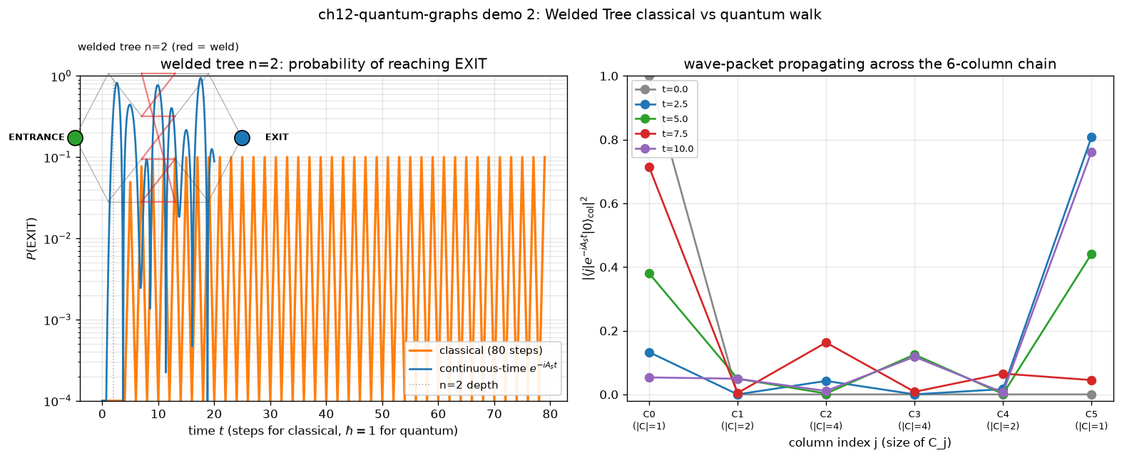
可视化：2 子图 —— 14 顶点焊缝树 + 经典 vs 量子 P(EXIT)

对应教程：第 12 章 量子图算法 中相关小节 · 依赖安装：pip install "unified-quantum[visualization,simulation]"

实现要点

核心：取 n=2 的焊接树 (2n+2=6 列、14 顶点)。左侧三列大小 1,2,4；右侧三列 大小 4,2,1；焊接在第 2 与第 3 列之间。整图邻接矩阵 A 在列子空间上压缩成 一条带权路径（边权树内 √2、焊缝 2）。连续时间量子游走 e^{-iAt}|0⟩_col 在 这个 6 维子空间上演化，振幅沿链传播并在 O(n) 时间内到达 EXIT 列；经典 随机游走 P_t = T^t |ENTRANCE⟩ 受生日悖论下界 2^{Ω(n)} 限制。这里画 P(EXIT) vs t 的对比曲线 + 列链上的概率剖面演化。

完整源码

demos/ch12-quantum-graphs/02_welded_tree.py

"""
ch12-quantum-graphs demo 2: Welded Tree — classical vs continuous-time quantum walk

对应教程：chenzhaoyun.com/quantum-tutorial/ch12-quantum-graphs/welded-tree.html
核心：取 n=2 的焊接树 (2n+2=6 列、14 顶点)。左侧三列大小 1,2,4；右侧三列
     大小 4,2,1；焊接在第 2 与第 3 列之间。整图邻接矩阵 A 在列子空间上压缩成
     一条带权路径（边权树内 √2、焊缝 2）。连续时间量子游走 e^{-iAt}|0⟩_col 在
     这个 6 维子空间上演化，振幅沿链传播并在 O(n) 时间内到达 EXIT 列；经典
     随机游走 P_t = T^t |ENTRANCE⟩ 受生日悖论下界 2^{Ω(n)} 限制。这里画
     P(EXIT) vs t 的对比曲线 + 列链上的概率剖面演化。

依赖：pip install unified-quantum[visualization]
运行：python demos/ch12-quantum-graphs/02_welded_tree.py
"""
from __future__ import annotations

from pathlib import Path

import matplotlib
matplotlib.use("Agg")
import matplotlib.pyplot as plt
import numpy as np
from scipy.linalg import expm

OUT = Path(__file__).parent

# === 1. Build welded tree graph (n = 2, N = 14) ===
N_DEPTH = 2
N = 2 ** (N_DEPTH + 2) - 2          # 14
N_COLS = 2 * N_DEPTH + 2            # 6
COL_SIZES = [2 ** j if j <= N_DEPTH else 2 ** (2 * N_DEPTH + 1 - j)
             for j in range(N_COLS)]
COL_OFFSET = np.concatenate([[0], np.cumsum(COL_SIZES)])

A = np.zeros((N, N), dtype=int)
# Left tree (cols 0..N_DEPTH-1): each vertex in col j has 2 children in col j+1
for col in range(N_DEPTH):
    for v_local in range(COL_SIZES[col]):
        v = COL_OFFSET[col] + v_local
        for c in range(2):
            A[v, COL_OFFSET[col + 1] + 2 * v_local + c] = 1
# Right tree (cols N_DEPTH+1..N_COLS-2): each vertex in col j has 1 parent in col j+1
for col in range(N_DEPTH + 1, N_COLS - 1):
    for v_local in range(COL_SIZES[col]):
        v = COL_OFFSET[col] + v_local
        A[v, COL_OFFSET[col + 1] + v_local // 2] = 1
# Weld: each left leaf connects to 2 right leaves (cyclic pairing)
left_n = COL_SIZES[N_DEPTH]
right_n = COL_SIZES[N_DEPTH + 1]
for v_local in range(left_n):
    v = COL_OFFSET[N_DEPTH] + v_local
    for r in [v_local % right_n, (v_local + 1) % right_n]:
        A[v, COL_OFFSET[N_DEPTH + 1] + r] = 1
A = np.maximum(A, A.T)               # symmetrize

deg = A.sum(axis=1)
max_deg = int(deg.max())
assert max_deg == 3, f"welded tree should have max degree 3, got {max_deg}"

# === 2. Column-subspace 6×6 tridiagonal matrix (weights √2 except weld=2) ===
A_col = np.zeros((N_COLS, N_COLS))
for j in range(N_COLS - 1):
    w = 2.0 if j == N_DEPTH else np.sqrt(2.0)
    A_col[j, j + 1] = A_col[j + 1, j] = w

# === 3. Classical random walk on full graph (start at ENTRANCE = vertex 0) ===
T = A / deg[None, :]                  # transition matrix
T_MAX = 80
exit_probs_class = np.zeros(T_MAX)
p = np.zeros(N); p[0] = 1.0
EXIT_VERTEX = N - 1
for t in range(T_MAX):
    exit_probs_class[t] = p[EXIT_VERTEX]
    p = T @ p

# === 4. Continuous-time quantum walk |psi(t)> = e^{-i A_col t} |0>_col ===
T_QUANT_MAX = 20.0
N_QUANT_STEPS = 200
t_quant = np.linspace(0, T_QUANT_MAX, N_QUANT_STEPS)
exit_probs_quant = np.zeros(N_QUANT_STEPS)
profile_probs = np.zeros((N_QUANT_STEPS, N_COLS))
v0 = np.zeros(N_COLS); v0[0] = 1.0
for k, t in enumerate(t_quant):
    probs = np.abs(expm(-1j * A_col * t) @ v0) ** 2
    exit_probs_quant[k] = probs[-1]
    profile_probs[k] = probs

# === 5. uniqc sanity: ENTRANCE = |0000⟩ should be deterministic ===
print("ch12-quantum-graphs-demo-2: Welded Tree (n=2) classical vs quantum walk")
print(f"  N = {N} vertices, columns = {N_COLS}, column sizes = {COL_SIZES}")
print(f"  max degree = {max_deg} (welded-tree invariant)")
try:
    from uniqc import Circuit, submit_task, wait_for_result
    c = Circuit()
    for q in range(4):
        c.measure(q)
    r = wait_for_result(
        submit_task(circuit=c, backend="dummy:local:simulator", shots=100)
    )
    counts = r.counts
    top = max(counts, key=counts.get)
    print(f"  uniqc sanity: |ENTRANCE>=|0000> with p={counts[top]/sum(counts.values()):.2f}")
except Exception as e:
    print(f"  uniqc sanity skipped: {e}")


# === 6. matplotlib 可视化 ===
fig, (ax1, ax2) = plt.subplots(1, 2, figsize=(13.0, 5.2))

# Left: P(EXIT) vs time, classical (steps) vs quantum (continuous)
ax1.semilogy(np.arange(T_MAX), np.maximum(exit_probs_class, 1e-4),
             "-", color="#ff7f0e", lw=2.0, label=f"classical ({T_MAX} steps)")
ax1.semilogy(t_quant, np.maximum(exit_probs_quant, 1e-4),
             "-", color="#1f77b4", lw=1.6,
             label=r"continuous-time $e^{-iA_S t}$")
ax1.axvline(N_DEPTH, color="gray", ls=":", lw=1, alpha=0.6,
            label=f"n={N_DEPTH} depth")
ax1.set_ylim(1e-4, 1.0)
ax1.set_xlabel(r"time $t$ (steps for classical, $\hbar=1$ for quantum)")
ax1.set_ylabel(r"$P(\mathrm{EXIT})$")
ax1.set_title("welded tree n=2: probability of reaching EXIT")
ax1.grid(alpha=0.3, which="both")
ax1.legend(loc="lower right", fontsize=9, framealpha=0.9)

# Right: column-probability profiles at selected times (wave packet propagation)
profile_times = [0.0, 2.5, 5.0, 7.5, 10.0]
colors_prof = ["#888888", "#1f77b4", "#2ca02c", "#d62728", "#9467bd"]
for tk, col_t in zip(profile_times, colors_prof):
    probs = np.abs(expm(-1j * A_col * tk) @ v0) ** 2
    ax2.plot(np.arange(N_COLS), probs, "-o", color=col_t, lw=1.6, ms=7,
             label=f"t={tk:.1f}")
ax2.set_xticks(np.arange(N_COLS))
ax2.set_xticklabels([f"C{j}\n(|C|={COL_SIZES[j]})" for j in range(N_COLS)],
                    fontsize=8)
ax2.set_xlabel("column index j (size of C_j)")
ax2.set_ylabel(r"$|\langle j | e^{-iA_S t} | 0\rangle_\mathrm{col}|^2$")
ax2.set_title("wave-packet propagating across the 6-column chain")
ax2.set_ylim(-0.02, 1.0)
ax2.grid(alpha=0.3)
ax2.legend(loc="upper left", fontsize=8, framealpha=0.9)

# Inset: welded tree sketch
inset = fig.add_axes([0.04, 0.55, 0.18, 0.36])
inset.set_xlim(-0.5, N_COLS - 0.5)
inset.set_ylim(-2.0, 2.0)
inset.axis("off")
node_pos = {}
for col, size in enumerate(COL_SIZES):
    ys = np.linspace(-1.6, 1.6, size) if size > 1 else [0.0]
    for i, y_ in enumerate(ys):
        node_pos[COL_OFFSET[col] + i] = (col, y_)
for i in range(N):
    for j in range(i + 1, N):
        if A[i, j]:
            x0, y0 = node_pos[i]; x1, y1 = node_pos[j]
            is_weld = (node_pos[i][0] == N_DEPTH and node_pos[j][0] == N_DEPTH + 1)
            color, lw, alpha = ("#d62728", 1.4, 0.55) if is_weld else ("#444", 0.7, 0.45)
            inset.plot([x0, x1], [y0, y1], "-", color=color, lw=lw, alpha=alpha)
inset.scatter(*node_pos[0], s=160, c="#2ca02c", ec="black", zorder=5)
inset.text(-0.3, 0, "ENTRANCE", ha="right", va="center",
           fontsize=8, fontweight="bold")
inset.scatter(*node_pos[N - 1], s=160, c="#1f77b4", ec="black", zorder=5)
inset.text(N_COLS - 0.3, 0, "EXIT", ha="left", va="center",
           fontsize=8, fontweight="bold")
inset.set_title("welded tree n=2 (red = weld)", fontsize=9)

plt.suptitle("ch12-quantum-graphs demo 2: Welded Tree classical vs quantum walk",
             y=1.02)
plt.tight_layout()
out_path = OUT / "02_welded_tree.png"
plt.savefig(out_path, dpi=120, bbox_inches="tight")
plt.close()

# === 7. stdout 关键统计 ===
peak_idx = int(np.argmax(exit_probs_quant))
print(f"\n  classical: max P(EXIT) over {T_MAX} steps = "
      f"{exit_probs_class.max():.4e}")
print(f"  classical: P(EXIT) at step {N_DEPTH} = "
      f"{exit_probs_class[N_DEPTH]:.4e}")
print(f"  quantum  : peak P(EXIT)={exit_probs_quant[peak_idx]:.3f} at "
      f"t={t_quant[peak_idx]:.2f}")
print(f"  quantum  : P(EXIT) at t=π={np.pi:.2f} = "
      f"{exit_probs_quant[np.argmin(np.abs(t_quant - np.pi))]:.3f}")
print(f"  A_col eigvals (rad/s): "
      f"{np.sort(np.linalg.eigvalsh(A_col)).round(3).tolist()}")
print(f"  theoretical weld weight: 2.0, tree weight: sqrt(2)={np.sqrt(2):.4f}")
print(f"  PNG -> {out_path}")

运行结果

运行方式

# 仓库根目录执行；输出 PNG 到 demos/ch12-quantum-graphs/02_welded_tree.png，关键统计到 stdout
.venv/bin/python3 demos/ch12-quantum-graphs/02_welded_tree.py

---

← 本章演示 · ↑ 代码演示总索引 · ⌂ 教程门户