Demo 2：主特征向量

第 15 章 梯度、谱方法与量子机器学习 · 本章演示 · 代码演示总索引

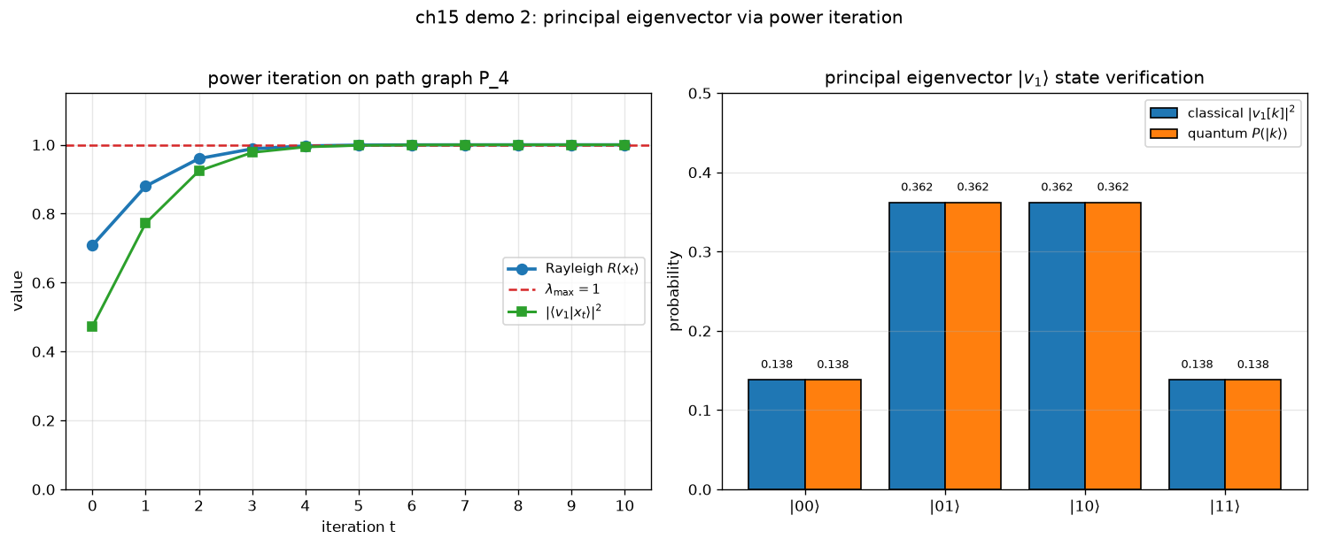
可视化：双图 —— 经典 power iter + 量子态制备

对应教程：第 15 章 梯度、谱方法与量子机器学习 中相关小节 · 依赖安装：pip install "unified-quantum[visualization,simulation]"

实现要点

核心: A 是 path graph P_4 的 adjacency matrix，归一化到 ||A||=1，主特征值 λ_max = 1.000。 经典 power iteration: x_t = A^t x_0 / ||...||，从 x_0 = (|00⟩+|01⟩)/√2 出发， Rayleigh 商 R(x_t) = ⟨x_t|A|x_t⟩ 单调收敛到 λ_max，|⟨v_1|x_t⟩|² 也 → 1。 量子端: 把收敛态 |v_1⟩ 用 5 个量子门 (H + 2·CNOT + RY + CNOT) 制备，再用 uniqc 测量 4 个基矢上的概率，验证与 numpy 算出的 v_1² 一致。这个 5-gate 分解依赖于 v_1 的对称性 (a=d, b=c)，所以中间连续两次 CNOT 等价于 swap-and-restore， 最后一个 CNOT 再 swap 一次即可得到目标。 uniqc 坑: get_matrix 不能在 measure 之后调用，所以验证在 measure 之前做。

完整源码

demos/ch15-learning-spectral/02_principal_eigenvector.py

"""
ch15 demo 2: principal eigenvector via (quantum) power iteration on path graph P_4

对应教程：chenzhaoyun.com/quantum-tutorial/ch15-learning-spectral/principal-eigenvector.html
核心: A 是 path graph P_4 的 adjacency matrix，归一化到 ||A||=1，主特征值 λ_max = 1.000。
     经典 power iteration: x_t = A^t x_0 / ||...||，从 x_0 = (|00⟩+|01⟩)/√2 出发，
     Rayleigh 商 R(x_t) = ⟨x_t|A|x_t⟩ 单调收敛到 λ_max，|⟨v_1|x_t⟩|² 也 → 1。
     量子端: 把收敛态 |v_1⟩ 用 5 个量子门 (H + 2·CNOT + RY + CNOT) 制备，再用 uniqc
  测量 4 个基矢上的概率，验证与 numpy 算出的 v_1² 一致。这个 5-gate 分解依赖于
  v_1 的对称性 (a=d, b=c)，所以中间连续两次 CNOT 等价于 swap-and-restore，
  最后一个 CNOT 再 swap 一次即可得到目标。
     uniqc 坑: get_matrix 不能在 measure 之后调用，所以验证在 measure 之前做。

依赖：pip install unified-quantum[visualization]
运行：python demos/ch15-learning-spectral/02_principal_eigenvector.py
"""
from __future__ import annotations

from pathlib import Path

import matplotlib
matplotlib.use("Agg")
import matplotlib.pyplot as plt
import numpy as np

from uniqc import Circuit, submit_task, wait_for_result

OUT = Path(__file__).parent
SHOTS = 1500

# === A: path graph P_4 adjacency + 0.5·I, normalized to spectral norm = 1 ===
# Adding 0.5·I shifts eigenvalues from {±1.618, ±0.618}/1.618 → {2.118, 1.118, -0.118, -1.118}/2.118
# = {1.0, 0.528, -0.056, -0.528}. λ_max is now unique and = 1, so power iteration
# converges cleanly to v_1 (no oscillation between λ_0 and λ_3 as in the bare path graph).
A_raw = np.array([
    [0.5, 1.0, 0.0, 0.0],
    [1.0, 0.5, 1.0, 0.0],
    [0.0, 1.0, 0.5, 1.0],
    [0.0, 0.0, 1.0, 0.5],
])
LAM_MAX_RAW = float(np.max(np.linalg.eigvalsh(A_raw)))
A = A_raw / LAM_MAX_RAW
LAM_MAX_NORM = 1.0

eigvals_full, eigvecs_full = np.linalg.eigh(A)
eigvals_sorted = eigvals_full[::-1]
V1 = eigvecs_full[:, -1].copy()
if V1[0] < 0:
    V1 = -V1

print("ch15-learning-spectral demo 2: principal eigenvector via power iteration")
print(f"  raw eigenvalues (path graph): {np.round(np.sort(np.linalg.eigvalsh(A_raw))[::-1], 4).tolist()}")
print(f"  normalized eigenvalues:      {np.round(eigvals_sorted, 4).tolist()}")
print(f"  λ_max (normalized) = {LAM_MAX_NORM:.4f}")
print(f"  v_1 = {np.round(V1, 4).tolist()}")

# === Classical power iteration from x_0 = (|00⟩ + |01⟩)/√2 ===
N_ITER = 10
x = np.array([1.0, 1.0, 0.0, 0.0], dtype=float) / np.sqrt(2.0)
rayleigh = []
overlap_v1 = []
for t in range(N_ITER + 1):
    norm_sq = float(np.dot(x, x))
    r = float(x @ A @ x) / norm_sq if norm_sq > 1e-12 else 0.0
    rayleigh.append(r)
    x_norm = x / np.sqrt(norm_sq) if norm_sq > 1e-12 else x
    overlap_v1.append(float(np.dot(V1, x_norm) ** 2))
    x = A @ x
    n = np.linalg.norm(x)
    if n < 1e-12:
        x = np.array([1.0, 1.0, 0.0, 0.0]) / np.sqrt(2.0)
    else:
        x = x / n

print(f"  Rayleigh R(x_t) over {N_ITER + 1} iterations:")
for t, (r, ov) in enumerate(zip(rayleigh, overlap_v1)):
    print(f"    t={t:2d}: R = {r:+.4f}  |⟨v_1|x_t⟩|² = {ov:.4f}")

# === Quantum: prepare |v_1⟩ via 5-gate decomposition and measure ===
# Use the symmetric structure: a=d, b=c, so 5-gate H+CNOT+CNOT+RY(α_1)+CNOT works
a, b, c, d = V1
alpha_1 = 2.0 * np.arctan2(b, a)  # RY on q1 to make q1 in (a|0⟩+b|1⟩)/√(a²+b²)
print(f"  state-prep RY angle: α_1 = {alpha_1:.4f}  (≈ 2·atan({b:.4f}/{a:.4f}))")

c_q = Circuit()
c_q.h(0)
c_q.cnot(0, 1)
c_q.cnot(0, 1)
c_q.ry(1, alpha_1)
c_q.cnot(0, 1)
c_q.barrier()
c_q.measure(0)
c_q.measure(1)

# Verify state prep before measure
c_check = Circuit()
c_check.h(0)
c_check.cnot(0, 1)
c_check.cnot(0, 1)
c_check.ry(1, alpha_1)
c_check.cnot(0, 1)
ref = np.array(c_check.get_matrix())
prepared = ref[:, 0]
err_prep = float(np.max(np.abs(np.abs(prepared) - V1)))
print(f"  state-prep max amplitude error: {err_prep:.4f}")
print(f"  circuit depth (with measure) = {c_q.depth}")

result = wait_for_result(submit_task(circuit=c_q, backend="dummy:local:simulator", shots=SHOTS))
counts = result.counts
total_shots = sum(max(0, v) for v in counts.values())

print(f"  measurement of |v_1⟩ ({total_shots} shots):")
quantum_probs = {}
for k in range(4):
    bs = format(k, "02b")
    cnt = counts.get(bs, 0)
    p = cnt / max(total_shots, 1)
    quantum_probs[k] = p
    print(f"    |{bs}⟩: {cnt:5d} shots  p = {p:.3f}  (classical |v_1[{k}]|² = {V1[k] ** 2:.3f})")

# === matplotlib 可视化 ===
fig, (ax1, ax2) = plt.subplots(1, 2, figsize=(12.5, 5.0))

# Left: convergence curves
t_arr = np.arange(N_ITER + 1)
ax1.plot(t_arr, rayleigh, "-o", color="#1f77b4", lw=2.2, ms=7,
         label=r"Rayleigh $R(x_t)$")
ax1.axhline(LAM_MAX_NORM, color="#d62728", ls="--", lw=1.5,
            label=r"$\lambda_{\max}=1$")
ax1.plot(t_arr, overlap_v1, "-s", color="#2ca02c", lw=1.8, ms=6,
         label=r"$|\langle v_1|x_t\rangle|^2$")
ax1.set_xticks(t_arr)
ax1.set_xlabel("iteration t")
ax1.set_ylabel("value")
ax1.set_ylim(0, 1.15)
ax1.set_title("power iteration on path graph P_4")
ax1.legend(loc="center right", fontsize=9)
ax1.grid(alpha=0.3)

# Right: |v_1⟩ verification (classical vs quantum)
x_idx = np.arange(4)
classical_v1_sq = V1 ** 2
quantum_v1_sq = np.array([quantum_probs[k] for k in range(4)])
ax2.bar(x_idx - 0.2, classical_v1_sq, 0.4, color="#1f77b4", ec="black",
        label=r"classical $|v_1[k]|^2$")
ax2.bar(x_idx + 0.2, quantum_v1_sq, 0.4, color="#ff7f0e", ec="black",
        label=r"quantum $P(|k\rangle)$")
for i in range(4):
    ax2.text(i - 0.2, classical_v1_sq[i] + 0.015, f"{classical_v1_sq[i]:.3f}",
             ha="center", fontsize=8)
    ax2.text(i + 0.2, quantum_v1_sq[i] + 0.015, f"{quantum_v1_sq[i]:.3f}",
             ha="center", fontsize=8)
ax2.set_xticks(x_idx)
ax2.set_xticklabels([f"|{k:02b}⟩" for k in range(4)])
ax2.set_ylabel("probability")
ax2.set_title(r"principal eigenvector $|v_1\rangle$ state verification")
ax2.set_ylim(0, 0.5)
ax2.legend(loc="upper right", fontsize=9)
ax2.grid(alpha=0.3, axis="y")

plt.suptitle("ch15 demo 2: principal eigenvector via power iteration", y=1.02)
plt.tight_layout()
out_path = OUT / "02_principal_eigenvector.png"
plt.savefig(out_path, dpi=120, bbox_inches="tight")
plt.close()

print()
print(f"  R(x_0) = {rayleigh[0]:.4f},  R(x_{N_ITER}) = {rayleigh[-1]:.4f}")
print(f"  |⟨v_1|x_0⟩|² = {overlap_v1[0]:.4f},  |⟨v_1|x_{N_ITER}⟩|² = {overlap_v1[-1]:.4f}")
print(f"  state-prep max error: {err_prep:.4f}")
print(f"  PNG -> {out_path}")

运行结果

运行方式

# 仓库根目录执行；输出 PNG 到 demos/ch15-learning-spectral/02_principal_eigenvector.png，关键统计到 stdout
.venv/bin/python3 demos/ch15-learning-spectral/02_principal_eigenvector.py

---

← 本章演示 · ↑ 代码演示总索引 · ⌂ 教程门户