Demo 2：态层析

第 7 章 量子信息 · 本章演示 · 代码演示总索引

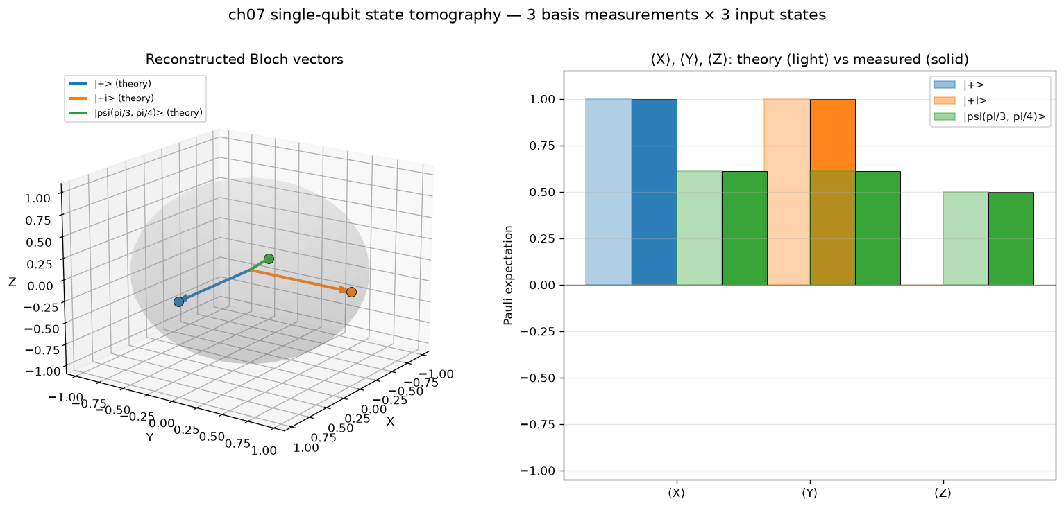
可视化：3D 球+3 子图 —— 3 态 3 基重建 Bloch 矢量

对应教程：第 7 章 量子信息 中相关小节 · 依赖安装：pip install "unified-quantum[visualization,simulation]"

实现要点

核心：对 3 个单 qubit 态做三轴 (X, Y, Z) 投影测量，重建 Bloch 矢量 并与理论值比较。

• |+> = H|0> (target Bloch: (1, 0, 0))

• |+i> = S·H|0> (target Bloch: (0, 1, 0))

• |psi_tt> = RY(pi/3) P(pi/4) |0> (general mixed-axis state)

测量约定：

• Z 基: 直接 measure(0)

• X 基: H(0) 后 measure，⟨X⟩ = 2·P(0) - 1

• Y 基: S†(0) H(0) 后 measure，⟨Y⟩ = 2·P(0) - 1

完整源码

demos/ch07-quantum-info/02_state_tomography.py

"""
ch07-quantum-info demo 2: single-qubit state tomography

对应教程：chenzhaoyun.com/quantum-tutorial/chch07-quantum-info/02-state-tomography.html
依赖：pip install unified-quantum[visualization]
运行：python demos/ch07-quantum-info/02_state_tomography.py

核心：对 3 个单 qubit 态做三轴 (X, Y, Z) 投影测量，重建 Bloch 矢量
并与理论值比较。
  - |+>         = H|0>          (target Bloch: (1, 0, 0))
  - |+i>        = S·H|0>        (target Bloch: (0, 1, 0))
  - |psi_tt>    = RY(pi/3) P(pi/4) |0>   (general mixed-axis state)

测量约定：
  - Z 基: 直接 measure(0)
  - X 基: H(0) 后 measure，⟨X⟩ = 2·P(0) - 1
  - Y 基: S†(0) H(0) 后 measure，⟨Y⟩ = 2·P(0) - 1
"""

from __future__ import annotations

from pathlib import Path

import matplotlib
matplotlib.use("Agg")
import matplotlib.pyplot as plt
import numpy as np

from uniqc import Circuit, submit_task, wait_for_result

OUT = Path(__file__).parent
SHOTS = 2000


# === 1. 单 qubit 三基态矢量期望测量 ===
def expectation_in_basis(state_prep, basis: str, shots: int = SHOTS) -> float:
    """对 state_prep 制备的态，在 basis (X/Y/Z) 上测 ⟨σ⟩ = 2·P(0) - 1。"""
    c = Circuit()
    state_prep(c)
    if basis == "X":
        c.h(0)
    elif basis == "Y":
        c.sdg(0)
        c.h(0)
    c.measure(0)
    r = wait_for_result(submit_task(c, backend="dummy:local:simulator", shots=shots))
    p0 = r.probabilities.get("0", 0.0)
    return 2.0 * p0 - 1.0


# === 2. 解析 Bloch 矢量 ===
def ry_p_state(theta: float, phi: float):
    """制备 RY(θ) P(φ) |0> = cos(θ/2)|0> + e^{iφ} sin(θ/2)|1>。"""
    def prep(c: Circuit) -> None:
        c.ry(0, theta)
        if phi != 0.0:
            c.p(0, phi)
    return prep


# === 3. 三个目标态 ===
def prep_plus(c: Circuit) -> None:
    c.h(0)


def prep_plus_i(c: Circuit) -> None:
    c.h(0)
    c.s(0)


PREPS = {
    "|+>": (prep_plus, np.array([1.0, 0.0, 0.0])),
    "|+i>": (prep_plus_i, np.array([0.0, 1.0, 0.0])),
    "|psi(pi/3, pi/4)>": (ry_p_state(np.pi / 3, np.pi / 4),
                    np.array([np.sin(np.pi / 3) * np.cos(np.pi / 4),
                              np.sin(np.pi / 3) * np.sin(np.pi / 4),
                              np.cos(np.pi / 3)])),
}


# === 4. 扫描每个态的 ⟨X⟩ ⟨Y⟩ ⟨Z⟩ ===
print("ch07-quantum-info demo 2: single-qubit state tomography")
results_table: dict[str, dict] = {}
bloch_measured = np.zeros((len(PREPS), 3))
bloch_theory = np.zeros((len(PREPS), 3))
labels = list(PREPS.keys())

for idx, (name, (prep_fn, theory)) in enumerate(PREPS.items()):
    bloch_theory[idx] = theory
    exps = []
    for j, basis in enumerate(["X", "Y", "Z"]):
        val = expectation_in_basis(prep_fn, basis, shots=SHOTS)
        exps.append(val)
    bloch_measured[idx] = np.array(exps)
    results_table[name] = {
        "measured": bloch_measured[idx],
        "theory": bloch_theory[idx],
    }
    print(f"  {name:24s}  theory = ({theory[0]:+.3f}, {theory[1]:+.3f}, {theory[2]:+.3f})  "
          f"measured = ({bloch_measured[idx, 0]:+.3f}, "
          f"{bloch_measured[idx, 1]:+.3f}, {bloch_measured[idx, 2]:+.3f})")

# 保真度 F = (1 + n_a · n_b) / 2，n 为 Bloch 矢量（纯态）
print()
for name, d in results_table.items():
    fid = 0.5 * (1.0 + float(d["theory"] @ d["measured"]))
    err = float(np.linalg.norm(d["measured"] - d["theory"]))
    print(f"  {name:24s}  F = {fid:.4f}  ||meas-theory|| = {err:.4f}")


# === 5. 画 2 子图 ===
fig = plt.figure(figsize=(13.0, 6.0))
ax_left = fig.add_subplot(1, 2, 1, projection="3d")
ax_right = fig.add_subplot(1, 2, 2)

colors = ["#1f77b4", "#ff7f0e", "#2ca02c"]

# 左图：Bloch sphere 上的理论 vs 测量矢量
u, v = np.mgrid[0:2 * np.pi:40j, 0:np.pi:20j]
xs = np.cos(u) * np.sin(v)
ys = np.sin(u) * np.sin(v)
zs = np.cos(v)
ax_left.plot_surface(xs, ys, zs, color="#dddddd", alpha=0.15, linewidth=0)
ax_left.set_xlim(-1.1, 1.1)
ax_left.set_ylim(-1.1, 1.1)
ax_left.set_zlim(-1.1, 1.1)
ax_left.set_xlabel("X")
ax_left.set_ylabel("Y")
ax_left.set_zlabel("Z")
ax_left.set_title("Reconstructed Bloch vectors", fontsize=12)
ax_left.view_init(elev=18, azim=35)

origin = np.zeros(3)
for i, (lab, c) in enumerate(zip(labels, colors)):
    th = bloch_theory[i]
    me = bloch_measured[i]
    ax_left.quiver(*origin, th[0], th[1], th[2], color=c, arrow_length_ratio=0.12,
                   linewidth=2.4, label=f"{lab} (theory)")
    ax_left.quiver(*th, me[0] - th[0], me[1] - th[1], me[2] - th[2],
                   color="black", arrow_length_ratio=0.18, linewidth=1.5,
                   linestyle="--")
    # 终点标记
    ax_left.scatter(*me, color=c, s=70, marker="o", edgecolor="black",
                    linewidth=0.6, zorder=10)
ax_left.legend(loc="upper left", bbox_to_anchor=(0.05, 1.0), fontsize=8)

# 右图：每个态在三个基上的 ⟨σ⟩，theory vs measured 双柱
axes_labels = ["⟨X⟩", "⟨Y⟩", "⟨Z⟩"]
x = np.arange(len(axes_labels))
width = 0.34
for i, (lab, c) in enumerate(zip(labels, colors)):
    offset = (i - 1) * width
    theory_bars = ax_right.bar(x + offset - width / 2, bloch_theory[i],
                                width, color=c, alpha=0.35,
                                edgecolor=c, linewidth=1.2,
                                label=f"{lab} (theory)" if i == 0 else None)
    meas_bars = ax_right.bar(x + offset + width / 2, bloch_measured[i],
                              width, color=c, alpha=0.95,
                              edgecolor="black", linewidth=0.6,
                              label=f"{lab} (measured)" if i == 0 else None)
ax_right.axhline(0, color="#888", lw=0.8)
ax_right.set_xticks(x)
ax_right.set_xticklabels(axes_labels)
ax_right.set_ylim(-1.05, 1.15)
ax_right.set_ylabel("Pauli expectation")
ax_right.set_title("⟨X⟩, ⟨Y⟩, ⟨Z⟩: theory (light) vs measured (solid)", fontsize=12)
ax_right.grid(axis="y", alpha=0.3)

# 一次性 legend 显示三个态
from matplotlib.patches import Patch
from matplotlib.lines import Line2D
legend_handles = []
for i, lab in enumerate(labels):
    legend_handles.append(Patch(facecolor=colors[i], alpha=0.45,
                                edgecolor=colors[i], label=f"{lab}"))
ax_right.legend(handles=legend_handles, loc="upper right", fontsize=9)

plt.suptitle("ch07 single-qubit state tomography — 3 basis measurements × 3 input states",
             fontsize=13, y=1.01)
plt.tight_layout()
out = OUT / "02_state_tomography.png"
plt.savefig(out, dpi=120, bbox_inches="tight")
plt.close()

print(f"  PNG -> {out}")

运行结果

运行方式

# 仓库根目录执行；输出 PNG 到 demos/ch07-quantum-info/02_state_tomography.png，关键统计到 stdout
.venv/bin/python3 demos/ch07-quantum-info/02_state_tomography.py

---

← 本章演示 · ↑ 代码演示总索引 · ⌂ 教程门户