Demo 1：QAOA K4 MaxCut

第 14 章 优化与数值量子算法 · 本章演示 · 代码演示总索引

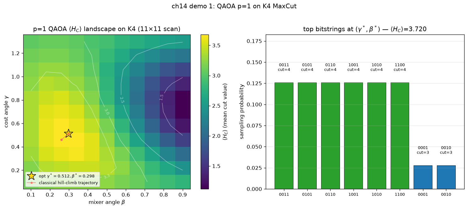
可视化：双图（热图+top cuts） —— 11×11 网格 + 爬山

对应教程：第 14 章 优化与数值量子算法 中相关小节 · 依赖安装：pip install "unified-quantum[visualization,simulation]"

实现要点

核心：K4 = 4-node complete graph, 6 edges. We scan the (γ, β) landscape for p=1 QAOA, plot ⟨H_C⟩ as a contour/heatmap, overlay a classical hill-climb trajectory that pushes past the grid optimum, then histogram the dominant bitstrings at the final (γ*, β*). For K4 the optimal cut = 4 and QAOA p=1 typically attains ≈ 0.92 approximation ratio (Farhi et al. 2014).

完整源码

demos/ch14-optimization-numerics/01_qaoa_maxcut_4node.py

"""
ch14-optimization-numerics demo 1: QAOA p=1 on the 4-node MaxCut (K4)

对应教程：chenzhaoyun.com/quantum-tutorial/ch14-optimization-numerics/constraint-satisfaction.html
核心：K4 = 4-node complete graph, 6 edges. We scan the (γ, β) landscape for
     p=1 QAOA, plot ⟨H_C⟩ as a contour/heatmap, overlay a classical hill-climb
     trajectory that pushes past the grid optimum, then histogram the dominant
     bitstrings at the final (γ*, β*). For K4 the optimal cut = 4 and QAOA p=1
     typically attains ≈ 0.92 approximation ratio (Farhi et al. 2014).

依赖：pip install unified-quantum[visualization]
运行：python demos/ch14-optimization-numerics/01_qaoa_maxcut_4node.py
"""
from __future__ import annotations

from pathlib import Path

import matplotlib
matplotlib.use("Agg")
import matplotlib.pyplot as plt
import numpy as np

from uniqc import qaoa_ansatz, submit_task, wait_for_result

OUT = Path(__file__).parent

# === 1. K4 graph and problem Hamiltonian ===
EDGES = [(0, 1), (0, 2), (0, 3), (1, 2), (1, 3), (2, 3)]
N_QUBITS = 4
OPT_CUT = 4

# Cost H_C = sum_edges (1 - Z_i Z_j)/2  →  drop the +1/2 constant, encode
# the Z_i Z_j part so that the sampler emits high-energy bitstrings when
# edges disagree.
H_C = [(f"Z{i}Z{j}", -0.5) for i, j in EDGES]

SHOTS = 600


def cut_value(bs: str) -> int:
    bs = bs.zfill(N_QUBITS)
    return sum(
        1 for i, j in EDGES
        if int(bs[N_QUBITS - 1 - i]) != int(bs[N_QUBITS - 1 - j])
    )


def evaluate_qaoa(gamma: float, beta: float, shots: int = SHOTS) -> float:
    c = qaoa_ansatz(H_C, p=1, gammas=np.array([gamma]), betas=np.array([beta]))
    for q in range(N_QUBITS):
        c.measure(q)
    r = wait_for_result(
        submit_task(circuit=c, backend="dummy:local:simulator", shots=shots)
    )
    counts = r.counts
    total = sum(counts.values())
    if total <= 0:
        return 0.0
    return sum(cut_value(bs) * cnt for bs, cnt in counts.items()) / total


def best_counts(gamma: float, beta: float, shots: int) -> dict:
    c = qaoa_ansatz(H_C, p=1, gammas=np.array([gamma]), betas=np.array([beta]))
    for q in range(N_QUBITS):
        c.measure(q)
    r = wait_for_result(
        submit_task(circuit=c, backend="dummy:local:simulator", shots=shots)
    )
    return r.counts


# === 2. γ × β landscape scan ===
print("ch14-demo-1: QAOA p=1 on K4 MaxCut")
print(f"  nodes={N_QUBITS}, edges={len(EDGES)}, optimal cut={OPT_CUT}")
print(f"  shots per QAOA run: {SHOTS}")

G = np.linspace(0.10, 1.30, 11)
B = np.linspace(0.10, 0.90, 11)
landscape = np.zeros((len(G), len(B)))
for gi, g in enumerate(G):
    for bi, b in enumerate(B):
        landscape[gi, bi] = evaluate_qaoa(g, b)
print(f"  grid scan: {len(G)} x {len(B)} = {len(G) * len(B)} points")

# === 3. classical hill-climb refinement ===
gi0, bi0 = np.unravel_index(int(np.argmax(landscape)), landscape.shape)
g_star, b_star = float(G[gi0]), float(B[bi0])
c_star = float(landscape[gi0, bi0])
trajectory = [(g_star, b_star, c_star)]

rng = np.random.default_rng(0)
for step in range(15):
    sigma = max(0.04, 0.18 * (0.55 ** step))
    g_try = float(np.clip(g_star + rng.normal(0, sigma), 0.05, np.pi))
    b_try = float(np.clip(b_star + rng.normal(0, sigma), 0.05, np.pi))
    c_try = evaluate_qaoa(g_try, b_try)
    if c_try > c_star:
        g_star, b_star, c_star = g_try, b_try, c_try
    trajectory.append((g_star, b_star, c_star))

# Big shots at optimum for the histogram
counts = best_counts(g_star, b_star, shots=4000)
hist = {bs.zfill(N_QUBITS): cnt for bs, cnt in counts.items()}
total_best = sum(hist.values())
hist_sorted = sorted(hist.items(), key=lambda kv: -kv[1])
top_states = hist_sorted[:8]

# === 4. visualisation ===
fig = plt.figure(figsize=(12.5, 5.4))
gs = fig.add_gridspec(1, 2, width_ratios=[1.05, 1.0])

# Left: landscape with hill-climb trajectory
ax1 = fig.add_subplot(gs[0, 0])
im = ax1.imshow(
    landscape, origin="lower", aspect="auto", cmap="viridis",
    extent=[B[0] - (B[1] - B[0]) / 2, B[-1] + (B[1] - B[0]) / 2,
            G[0] - (G[1] - G[0]) / 2, G[-1] + (G[1] - G[0]) / 2],
)
cs = ax1.contour(B, G, landscape, levels=[1.5, 2.5, 3.0, 3.3],
                 colors="white", linewidths=0.7, alpha=0.55)
ax1.clabel(cs, inline=True, fontsize=8, fmt="%.1f")
ax1.plot([b_star], [g_star], "*", color="#ffd700", ms=18, mec="black", mew=0.9,
         label=rf"opt $\gamma^*={g_star:.3f},\beta^*={b_star:.3f}$")
traj_g = [t[0] for t in trajectory]
traj_b = [t[1] for t in trajectory]
ax1.plot(traj_b, traj_g, "-o", color="#ff6f61", ms=3, lw=1.0, alpha=0.8,
         label="classical hill-climb trajectory")
ax1.set_xlabel(r"mixer angle $\beta$")
ax1.set_ylabel(r"cost angle $\gamma$")
ax1.set_title(r"p=1 QAOA $\langle H_C\rangle$ landscape on K4 (11×11 scan)")
cbar = plt.colorbar(im, ax=ax1)
cbar.set_label(r"$\langle H_C\rangle$ (mean cut value)")
ax1.legend(loc="lower left", fontsize=8)

# Right: top bitstrings histogram
ax2 = fig.add_subplot(gs[0, 1])
labels = [bs for bs, _ in top_states]
probs = [cnt / total_best for _, cnt in top_states]
cuts = [cut_value(bs) for bs, _ in top_states]
colors = ["#2ca02c" if c == OPT_CUT else
          "#1f77b4" if c == OPT_CUT - 1 else "#d62728" for c in cuts]
bars = ax2.bar(range(len(labels)), probs, color=colors, ec="black", lw=0.5)
for k, (lab, p, c) in enumerate(zip(labels, probs, cuts)):
    ax2.text(k, p + 0.012, f"{lab}\ncut={c}", ha="center", va="bottom",
             fontsize=7.5)
ax2.set_xticks(range(len(labels)))
ax2.set_xticklabels(labels, rotation=0, fontsize=8)
ax2.set_ylabel("sampling probability")
ax2.set_title(rf"top bitstrings at $(\gamma^*,\beta^*)$ — $\langle H_C\rangle$={c_star:.3f}")
ax2.set_ylim(0, max(probs) * 1.45)
ax2.grid(alpha=0.3, axis="y")

plt.suptitle("ch14 demo 1: QAOA p=1 on K4 MaxCut", y=1.02)
plt.tight_layout()
out_path = OUT / "01_qaoa_maxcut_4node.png"
plt.savefig(out_path, dpi=120, bbox_inches="tight")
plt.close()

# === 5. stdout 关键统计 ===
total_evals = len(G) * len(B) + len(trajectory) - 1 + 1
print(f"  total QAOA circuit evaluations: {total_evals}")
print(f"  grid best      : cuts={float(landscape.max()):.3f}/{OPT_CUT} "
      f"at γ={G[gi0]:.3f}, β={B[bi0]:.3f}")
print(f"  after hill-climb: γ*={g_star:.4f}, β*={b_star:.4f}")
print(f"  mean cut value  : {c_star:.4f} / {OPT_CUT}")
print(f"  approximation r : {c_star / OPT_CUT:.4f}  (3-regular worst-case guarantee = 0.6924)")
print(f"  top 4 bitstrings:")
for bs, cnt in hist_sorted[:4]:
    print(f"    |{bs}>  cut={cut_value(bs)}  p={cnt/total_best:.4f}")
print(f"  PNG -> {out_path}")

运行结果

运行方式

# 仓库根目录执行；输出 PNG 到 demos/ch14-optimization-numerics/01_qaoa_maxcut_4node.png，关键统计到 stdout
.venv/bin/python3 demos/ch14-optimization-numerics/01_qaoa_maxcut_4node.py

---

← 本章演示 · ↑ 代码演示总索引 · ⌂ 教程门户