Demo 3：量子核 SVM

第 8 章 量子机器学习 · 本章演示 · 代码演示总索引

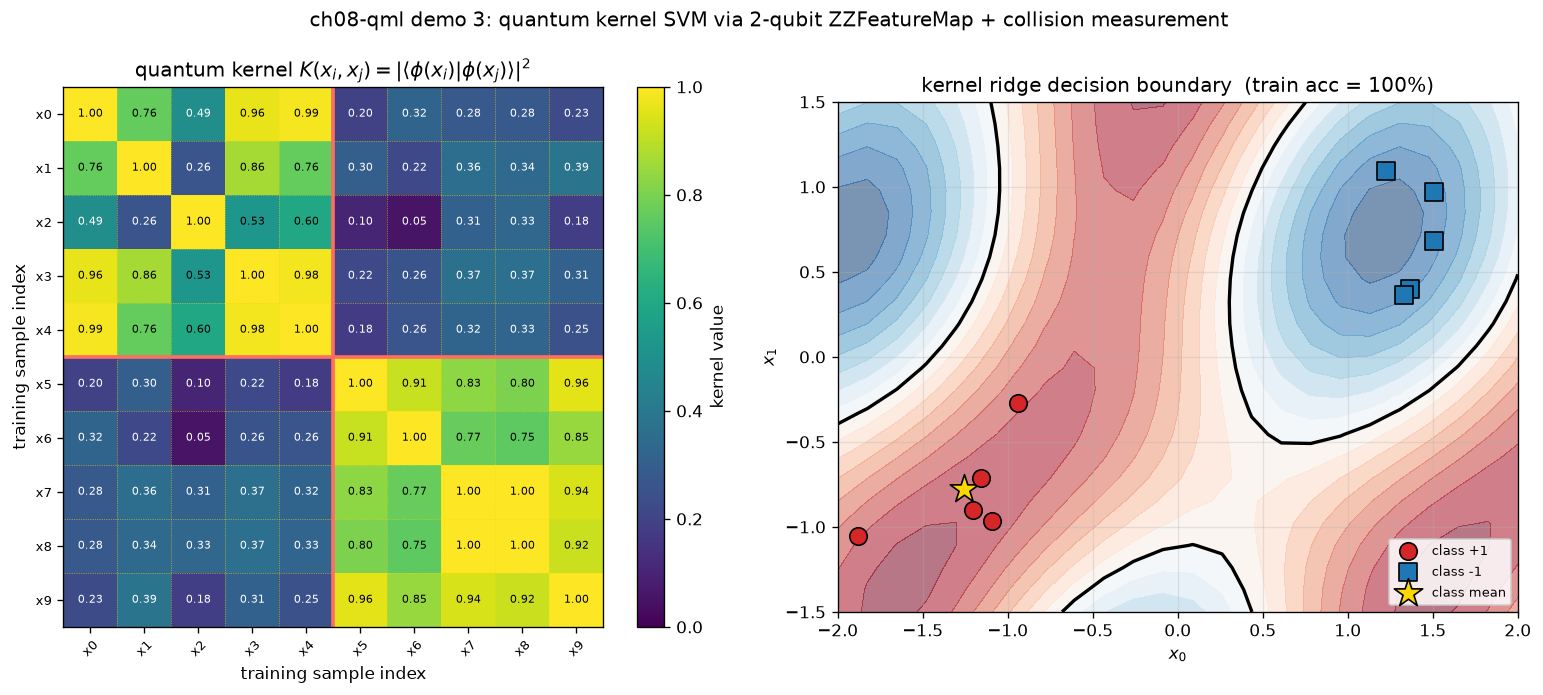
可视化：双图（核矩阵+边界） —— 2-qubit ZZFeatureMap 核矩阵 + 决策边界

对应教程：第 8 章 量子机器学习 中相关小节 · 依赖安装：pip install "unified-quantum[visualization,simulation]"

实现要点

核心：用 2-qubit ZZFeatureMap U_φ(x) = (H⊗H) · [RZ(x_0)⊗RZ(x_1)] · CNOT · [RZ(x_0)⊗RZ(x_1)] 编码 2D 数据点，通过碰撞测量 K(x,x') = Pr(|00⟩) on circuit U_φ(x')^dagger · U_φ(x) |00⟩ = |⟨φ(x)|φ(x')⟩|² 估计训练集两两核矩阵 K。然后用核岭回归（kernel ridge regression, 闭合解）在核矩阵上加 λI 求逆，得到分类器 f(x) = K(x, X_train) · (K_train + λI)^{-1} · y_train 绘制核矩阵热图 + 二维决策边界。

完整源码

demos/ch08-qml/03_quantum_kernel.py

"""
ch08-qml demo 3: Quantum kernel via 2-qubit ZZFeatureMap

对应教程：chenzhaoyun.com/quantum-tutorial/ch08-qml/quantum-kernel.html
核心：用 2-qubit ZZFeatureMap
        U_φ(x) = (H⊗H) · [RZ(x_0)⊗RZ(x_1)] · CNOT · [RZ(x_0)⊗RZ(x_1)]
     编码 2D 数据点，通过碰撞测量
        K(x,x') = Pr(|00⟩) on circuit U_φ(x')^dagger · U_φ(x) |00⟩
                  = |⟨φ(x)|φ(x')⟩|²
     估计训练集两两核矩阵 K。然后用核岭回归（kernel ridge regression,
     闭合解）在核矩阵上加 λI 求逆，得到分类器
        f(x) = K(x, X_train) · (K_train + λI)^{-1} · y_train
     绘制核矩阵热图 + 二维决策边界。

依赖：pip install unified-quantum[visualization] scipy
运行：python demos/ch08-qml/03_quantum_kernel.py
"""
from __future__ import annotations

from pathlib import Path

import matplotlib
matplotlib.use("Agg")
import matplotlib.pyplot as plt
import numpy as np

from uniqc import Circuit, submit_task, wait_for_result

OUT = Path(__file__).parent

SHOTS = 2000
N_QUBITS = 2


def zzfm(x0: float, x1: float, dagger: bool = False) -> Circuit:
    """ZZFeatureMap on 2 qubits, optional dagger."""
    c = Circuit()
    if dagger:
        c.rz(0, float(-x0)); c.rz(1, float(-x1))
        c.cnot(0, 1)
        c.rz(0, float(-x0)); c.rz(1, float(-x1))
        c.h(0); c.h(1)
    else:
        c.h(0); c.h(1)
        c.rz(0, float(x0)); c.rz(1, float(x1))
        c.cnot(0, 1)
        c.rz(0, float(x0)); c.rz(1, float(x1))
    return c


def quantum_kernel(x: np.ndarray, x_prime: np.ndarray, shots: int = SHOTS) -> float:
    """Collision-measurement estimate of K(x, x') = |⟨φ(x)|φ(x')⟩|²."""
    c = Circuit()
    c.add_circuit(zzfm(float(x[0]), float(x[1]), dagger=False))
    c.add_circuit(zzfm(float(x_prime[0]), float(x_prime[1]), dagger=True))
    c.measure(0); c.measure(1)
    r = wait_for_result(submit_task(circuit=c, backend="dummy:local:simulator", shots=shots))
    return float(r.probabilities.get("00", 0.0))


def kernel_matrix(X: np.ndarray, shots: int = SHOTS) -> np.ndarray:
    """Pairwise quantum kernel matrix K[i, j] = |⟨φ(x_i)|φ(x_j)⟩|²."""
    n = len(X)
    K = np.eye(n)
    for i in range(n):
        for j in range(i + 1, n):
            k = quantum_kernel(X[i], X[j], shots=shots)
            K[i, j] = k
            K[j, i] = k
    return K


# === 1. Toy 2-D bimodal dataset ===
rng = np.random.default_rng(42)
# class +1: cluster around (-π/2, -π/4); class -1: cluster around (+π/2, +π/2)
n_per_class = 5
X_pos = rng.normal(loc=[-1.2, -0.6], scale=0.35, size=(n_per_class, 2))
X_neg = rng.normal(loc=[+1.2, +0.7], scale=0.35, size=(n_per_class, 2))
X_train = np.vstack([X_pos, X_neg])
y_train = np.array([+1] * n_per_class + [-1] * n_per_class, dtype=float)
N_TRAIN = len(X_train)

print("ch08-qml-demo-3: quantum kernel SVM via 2-qubit ZZFeatureMap")
print(f"  training samples: {N_TRAIN}  ({n_per_class} per class)")
print(f"  feature dimension: {X_train.shape[1]}")
print(f"  shots per kernel value: {SHOTS}")


# === 2. Quantum kernel matrix via collision measurements ===
n_pairs = N_TRAIN * (N_TRAIN + 1) // 2
print(f"  computing {n_pairs} pairwise kernel values via quantum collision...")
K_quantum = kernel_matrix(X_train, shots=SHOTS)


# === 3. Train a kernel ridge regression classifier (closed-form α) ===
LAMBDA = 0.10
alpha = np.linalg.solve(K_quantum + LAMBDA * np.eye(N_TRAIN), y_train)


def predict_kernel_ridge(X_query: np.ndarray) -> np.ndarray:
    """f(x) = K(x, X_train) @ alpha; threshold at 0 for binary class."""
    n_query = len(X_query)
    f_vals = np.zeros(n_query)
    for k in range(n_query):
        k_row = np.array([quantum_kernel(X_query[k], X_train[i], shots=SHOTS) for i in range(N_TRAIN)])
        f_vals[k] = float(k_row @ alpha)
    return f_vals


# === 4. Sanity: train accuracy ===
f_train = np.array([K_quantum[i] @ alpha for i in range(N_TRAIN)])
train_acc = float(np.mean(np.sign(f_train) == y_train))

# === 5. Decision boundary on a 2-D grid ===
GRID = 24
grid_x = np.linspace(-2.0, 2.0, GRID)
grid_y = np.linspace(-1.5, 1.5, GRID)
XX, YY = np.meshgrid(grid_x, grid_y)
grid_points = np.column_stack([XX.ravel(), YY.ravel()])

print(f"  evaluating decision boundary on {GRID}x{GRID} = {len(grid_points)} grid points...")
Z = predict_kernel_ridge(grid_points).reshape(XX.shape)


# === 6. matplotlib 可视化 ===
fig, (ax1, ax2) = plt.subplots(1, 2, figsize=(13.0, 5.4))

# Left: kernel matrix heatmap
im = ax1.imshow(K_quantum, cmap="viridis", vmin=0.0, vmax=1.0, origin="upper")
ax1.set_xticks(range(N_TRAIN))
ax1.set_yticks(range(N_TRAIN))
ax1.set_xticklabels([f"x{i}" for i in range(N_TRAIN)], fontsize=8, rotation=45)
ax1.set_yticklabels([f"x{i}" for i in range(N_TRAIN)], fontsize=8)
for i in range(N_TRAIN):
    for j in range(N_TRAIN):
        ax1.text(j, i, f"{K_quantum[i, j]:.2f}",
                 ha="center", va="center", fontsize=6.5,
                 color="white" if K_quantum[i, j] < 0.5 else "black")
# colour class boundaries on the heatmap
for i in range(N_TRAIN):
    ax1.axhline(i + 0.5, color="#ffd700", lw=0.4, ls=":")
    ax1.axvline(i + 0.5, color="#ffd700", lw=0.4, ls=":")
    ax1.axhline(n_per_class - 0.5, color="#ff6f61", lw=1.4)
    ax1.axvline(n_per_class - 0.5, color="#ff6f61", lw=1.4)
ax1.set_xlabel("training sample index")
ax1.set_ylabel("training sample index")
ax1.set_title(r"quantum kernel $K(x_i, x_j) = |\langle\phi(x_i)|\phi(x_j)\rangle|^2$")
cbar = plt.colorbar(im, ax=ax1)
cbar.set_label(r"kernel value")

# Right: decision boundary + training points
ax2.contourf(XX, YY, Z, levels=20, cmap="RdBu_r", alpha=0.55)
ax2.contour(XX, YY, Z, levels=[0.0], colors="black", linewidths=2.0)
# training data
for cls, marker, color, label in [
    (+1, "o", "#d62728", "class +1"),
    (-1, "s", "#1f77b4", "class -1"),
]:
    idx = (y_train == cls)
    ax2.scatter(X_train[idx, 0], X_train[idx, 1], s=110, marker=marker,
                ec="black", color=color, zorder=5, label=label)
# mark class centers
ax2.scatter(*X_pos.mean(axis=0), s=320, marker="*", ec="black",
            fc="#ffd700", zorder=4, label="class mean")
ax2.set_xlabel(r"$x_0$")
ax2.set_ylabel(r"$x_1$")
ax2.set_title(
    fr"kernel ridge decision boundary  (train acc = {train_acc*100:.0f}%)"
)
ax2.legend(loc="lower right", fontsize=8, framealpha=0.85)
ax2.grid(alpha=0.3)
ax2.set_aspect("equal", adjustable="box")

plt.suptitle(
    r"ch08-qml demo 3: quantum kernel SVM via 2-qubit ZZFeatureMap + collision measurement",
    y=1.02,
)
plt.tight_layout()
out_path = OUT / "03_quantum_kernel.png"
plt.savefig(out_path, dpi=120, bbox_inches="tight")
plt.close()


# === 7. stdout 关键统计 ===
print(f"  quantum kernel matrix K shape: {K_quantum.shape}")
print(f"  K[i, i] mean (should ≈ 1)    : {np.diag(K_quantum).mean():.4f}")
print(f"  K off-diagonal mean           : {(K_quantum.sum() - N_TRAIN)/(N_TRAIN*(N_TRAIN-1)):.4f}")
print(f"  K[+class, +class] mean        : {K_quantum[:n_per_class, :n_per_class].mean():.4f}")
print(f"  K[-class, -class] mean        : {K_quantum[n_per_class:, n_per_class:].mean():.4f}")
print(f"  K[+class, -class] mean        : {K_quantum[:n_per_class, n_per_class:].mean():.4f}")
print(f"  ridge regularization λ        : {LAMBDA}")
print(f"  train accuracy                : {train_acc*100:.1f}%")
print(f"  quantum circuit evaluations   : {n_pairs + len(grid_points)*N_TRAIN}")
print(f"  PNG -> {out_path}")

运行结果

运行方式

# 仓库根目录执行；输出 PNG 到 demos/ch08-qml/03_quantum_kernel.png，关键统计到 stdout
.venv/bin/python3 demos/ch08-qml/03_quantum_kernel.py

---

← 本章演示 · ↑ 代码演示总索引 · ⌂ 教程门户