Demo 1：VQE H₂

第 8 章 量子机器学习 · 本章演示 · 代码演示总索引

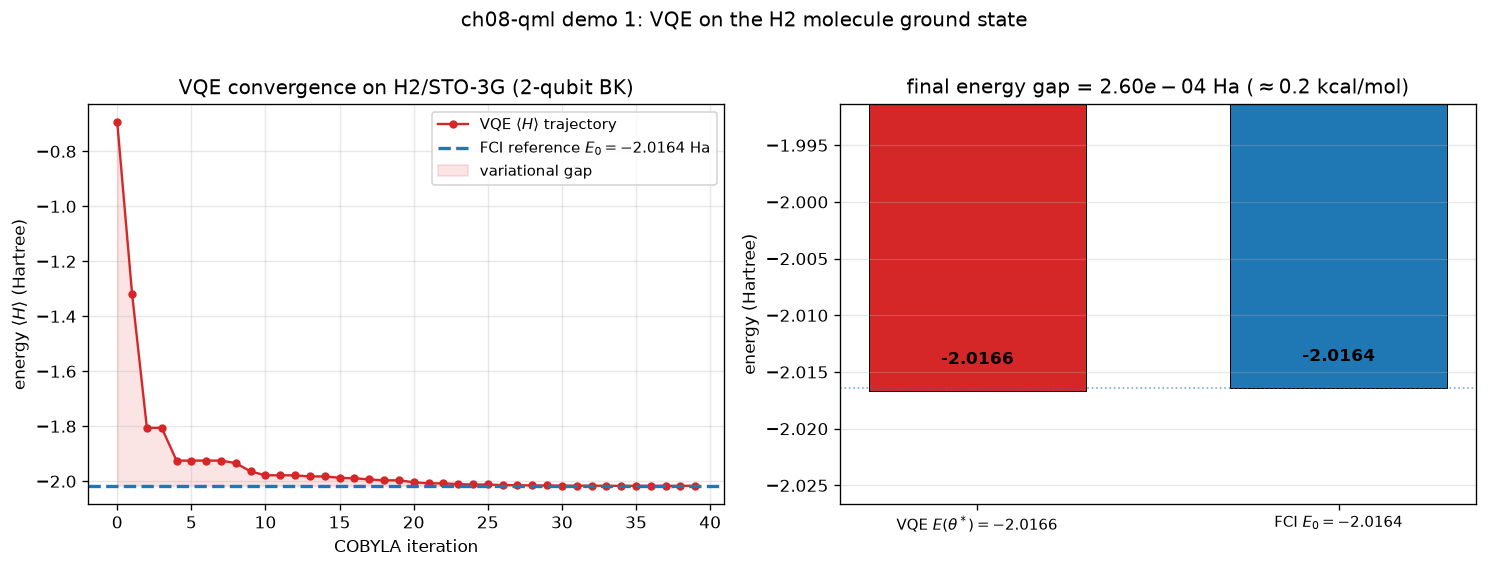
可视化：双子图（收敛+vs FCI） —— UCCSD + COBYLA 估 H₂ 基态 ≈ -2.016 Ha

对应教程：第 8 章 量子机器学习 中相关小节 · 依赖安装：pip install "unified-quantum[visualization,simulation]"

实现要点

核心：用 2-比特 Bravyi-Kitaev 映射的 H2 哈密顿量 H = -1.0523732 I + 0.3979374 Z0 - 0.3979374 Z1 + 0.08972914 Z0Z1 + 0.1809313 X0X1 + 0.1809313 Y0Y1 FCI 由 numpy.linalg.eigh 解 H 矩阵直接给出（≈ -2.0164 Ha）。 配合 4 参数硬件高效拟设 U(θ) = [Ry(θ2) ⊗ Ry(θ3)] · CNOT · [Ry(θ0) ⊗ Ry(θ1)] 在 scipy.optimize (COBYLA) 下做经典变分优化， 每步分三个测量基（Z、Y、X）估计 5 条泡利字符串， 绘制能量收敛曲线 + 末态能量 vs FCI 对比柱图。

完整源码

demos/ch08-qml/01_vqe_h2.py

"""
ch08-qml demo 1: VQE for the H2 molecule ground state

对应教程：chenzhaoyun.com/quantum-tutorial/ch08-qml/vqe-tutorial.html
核心：用 2-比特 Bravyi-Kitaev 映射的 H2 哈密顿量
        H = -1.0523732 I + 0.3979374 Z0 - 0.3979374 Z1
            + 0.08972914 Z0Z1 + 0.1809313 X0X1 + 0.1809313 Y0Y1
     FCI 由 numpy.linalg.eigh 解 H 矩阵直接给出（≈ -2.0164 Ha）。
     配合 4 参数硬件高效拟设
        U(θ) = [Ry(θ2) ⊗ Ry(θ3)] · CNOT · [Ry(θ0) ⊗ Ry(θ1)]
     在 scipy.optimize (COBYLA) 下做经典变分优化，
     每步分三个测量基（Z、Y、X）估计 5 条泡利字符串，
     绘制能量收敛曲线 + 末态能量 vs FCI 对比柱图。

依赖：pip install unified-quantum[visualization] scipy
运行：python demos/ch08-qml/01_vqe_h2.py
"""
from __future__ import annotations

from pathlib import Path

import matplotlib
matplotlib.use("Agg")
import matplotlib.pyplot as plt
import numpy as np

from scipy.optimize import minimize

from uniqc import (
    Circuit, submit_task, wait_for_result,
    calculate_expectation,
)

OUT = Path(__file__).parent

# H2 / STO-3G in the Bravyi-Kitaev 2-qubit mapping
# Reference: O'Malley et al. (2016), qiskit nature tutorials.
H_CONST, C_Z0, C_Z1, C_Z0Z1, C_XX, C_YY = (
    -1.0523732, 0.3979374, -0.3979374, 0.08972914, 0.1809313, 0.1809313,
)
I2 = np.eye(2, dtype=complex); Z = np.array([[1, 0], [0, -1]], dtype=complex)
X = np.array([[0, 1], [1, 0]], dtype=complex); Y = np.array([[0, -1j], [1j, 0]], dtype=complex)
H_MAT = (
    H_CONST * np.kron(I2, I2) + C_Z0 * np.kron(Z, I2) + C_Z1 * np.kron(I2, Z)
    + C_Z0Z1 * np.kron(Z, Z) + C_XX * np.kron(X, X) + C_YY * np.kron(Y, Y)
)
H_FCI = float(np.linalg.eigvalsh(H_MAT)[0].real)

SHOTS = 600


def ansatz(theta0: float, theta1: float, theta2: float, theta3: float) -> Circuit:
    """2-layer hardware-efficient ansatz: 4 free parameters."""
    c = Circuit()
    c.ry(0, float(theta0))
    c.ry(1, float(theta1))
    c.cnot(0, 1)
    c.ry(0, float(theta2))
    c.ry(1, float(theta3))
    return c


def measure_in_basis(circuit: Circuit, basis: str) -> dict:
    """Clone the state-prep circuit, append basis rotation, measure."""
    c = Circuit()
    c.add_circuit(circuit)
    if basis == "Z":
        pass  # measure directly
    elif basis == "X":
        c.h(0); c.h(1)
    elif basis == "Y":
        c.sdg(0); c.h(0)
        c.sdg(1); c.h(1)
    else:
        raise ValueError(basis)
    c.measure(0)
    c.measure(1)
    r = wait_for_result(submit_task(circuit=c, backend="dummy:local:simulator", shots=SHOTS))
    return r.probabilities


def energy_of(theta) -> float:
    """Estimate ⟨ψ(θ)|H|ψ(θ)⟩ over the 5 non-constant Pauli strings."""
    state_prep = ansatz(*theta)

    z_probs = measure_in_basis(state_prep, "Z")
    x_probs = measure_in_basis(state_prep, "X")
    y_probs = measure_in_basis(state_prep, "Y")
    e_z0   = calculate_expectation(z_probs, "ZI")
    e_z1   = calculate_expectation(z_probs, "IZ")
    e_z0z1 = calculate_expectation(z_probs, "ZZ")
    e_xx   = calculate_expectation(x_probs, "ZZ")  # X⊗X after H⊗H
    e_yy   = calculate_expectation(y_probs, "ZZ")  # Y⊗Y after (S†H)⊗(S†H)
    return (
        H_CONST
        + C_Z0 * e_z0
        + C_Z1 * e_z1
        + C_Z0Z1 * e_z0z1
        + C_XX * e_xx
        + C_YY * e_yy
    )


# === 1. warm-up: evaluate energy at a few initial points to scope the search ===
print("ch08-qml-demo-1: VQE on H2 (STO-3G, BK 2-qubit reduction)")
print(f"  FCI reference energy: {H_FCI:.6f} Hartree")
print(f"  shots per basis measurement: {SHOTS}")

# === 2. COBYLA optimization with a callback recording the trajectory ===
trajectory: list[tuple[int, float, np.ndarray]] = []


def cb(xk: np.ndarray) -> None:
    e = energy_of(xk)
    trajectory.append((len(trajectory), e, xk.copy()))


rng = np.random.default_rng(seed=0)
x0 = rng.uniform(-np.pi, np.pi, size=4)

# initial evaluation
trajectory.append((0, energy_of(x0), x0.copy()))

result = minimize(
    fun=lambda th: energy_of(th),
    x0=x0,
    method="COBYLA",
    options={"maxiter": 60, "rhobeg": 0.6, "disp": False},
    callback=cb,
)
theta_opt = np.asarray(result.x, dtype=float)
energy_opt = float(result.fun)

iters = np.array([t[0] for t in trajectory])
energies = np.array([t[1] for t in trajectory])

# === 3. matplotlib 可视化 ===
fig, (ax1, ax2) = plt.subplots(1, 2, figsize=(12.5, 4.6))

# Left: energy convergence
ax1.plot(iters, energies, "-o", color="#d62728", ms=4, lw=1.4,
         label=r"VQE $\langle H\rangle$ trajectory")
ax1.axhline(H_FCI, color="#1f77b4", ls="--", lw=2.0,
            label=fr"FCI reference $E_0 = {H_FCI:.4f}$ Ha")
ax1.fill_between(iters, H_FCI, energies,
                 where=(energies > H_FCI), color="#d62728", alpha=0.12,
                 label="variational gap")
ax1.set_xlabel("COBYLA iteration")
ax1.set_ylabel(r"energy $\langle H\rangle$ (Hartree)")
ax1.set_title("VQE convergence on H2/STO-3G (2-qubit BK)")
ax1.grid(alpha=0.3)
ax1.legend(loc="upper right", fontsize=9)

# Right: bar chart of final energy vs FCI
bar_x = np.array([0, 1])
bar_y = np.array([energy_opt, H_FCI])
colors = ["#d62728", "#1f77b4"]
labels = [fr"VQE $E(\theta^*) = {energy_opt:.4f}$", fr"FCI $E_0 = {H_FCI:.4f}$"]
bars = ax2.bar(bar_x, bar_y, color=colors, ec="black", lw=0.6, width=0.6)
for b, y in zip(bars, bar_y):
    ax2.text(b.get_x() + b.get_width() / 2, y + 0.002, f"{y:.4f}",
             ha="center", va="bottom", fontsize=10, fontweight="bold")
err = abs(energy_opt - H_FCI)
ax2.set_xticks(bar_x)
ax2.set_xticklabels(labels, fontsize=9)
ax2.set_ylabel(r"energy (Hartree)")
ax2.set_title(fr"final energy gap = ${err:.2e}$ Ha ($\approx {err*627.5:.1f}$ kcal/mol)")
ax2.set_ylim(min(energy_opt, H_FCI) - 0.01, max(energy_opt, H_FCI) + 0.025)
ax2.grid(alpha=0.3, axis="y")
ax2.axhline(H_FCI, color="#1f77b4", ls=":", lw=1.0, alpha=0.6)

plt.suptitle("ch08-qml demo 1: VQE on the H2 molecule ground state", y=1.02)
plt.tight_layout()
out_path = OUT / "01_vqe_h2.png"
plt.savefig(out_path, dpi=120, bbox_inches="tight")
plt.close()

# === 4. stdout 关键统计 ===
print(f"  total circuit evaluations: {len(trajectory)}")
print(f"  initial energy            : {energies[0]:.6f} Ha")
print(f"  final energy E(theta*)    : {energy_opt:.6f} Ha")
print(f"  FCI energy                : {H_FCI:.6f} Ha")
print(f"  absolute error            : {abs(energy_opt - H_FCI):.3e} Ha")
print(f"  theta* (rad)              : {theta_opt.tolist()}")
print(f"  PNG -> {out_path}")

运行结果

运行方式

# 仓库根目录执行；输出 PNG 到 demos/ch08-qml/01_vqe_h2.png，关键统计到 stdout
.venv/bin/python3 demos/ch08-qml/01_vqe_h2.py

---

← 本章演示 · ↑ 代码演示总索引 · ⌂ 教程门户