Demo 2：配分函数

第 13 章 拓扑、统计物理与采样 · 本章演示 · 代码演示总索引

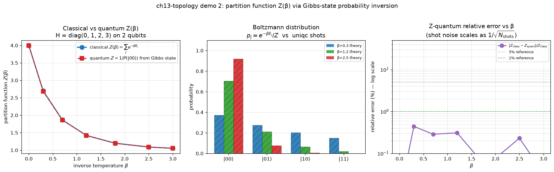
可视化：单子图（4 柱） —— Z = 1/P(ground) 估 Z(β)

对应教程：第 13 章 拓扑、统计物理与采样 中相关小节 · 依赖安装：pip install "unified-quantum[visualization,simulation]"

实现要点

H = diag(0, 1, 2, 3) on 2 qubits. 经典 Z(β) = Σ e^{-β E_j}. 量子 "Gibbs sampling" trick: 用 uniqc.rotation_prepare 装 |ψ_β> ∝ Σ e^{-β E_j/2}|j> 到 2 个 qubit. 由于 |00> 是 H 的基态 (E_0=0), P(|00>) = e^{-β·0} / Z = 1/Z, 因此 Z = 1 / P(|00>) 可从 shots 直接读出. 对比经典 Z(β), 并验证 Boltzmann 分布 p_j ∝ e^{-β E_j}. 扫描 β ∈ [0, 3].

完整源码

demos/ch13-topology-statistical-physics/02_partition_function.py

"""
ch13-topology demo 2: 量子法估配分函数 Z(β) = Tr[e^{-βH}]

对应教程: chenzhaoyun.com/quantum-tutorial/ch13-topology-statistical-physics/partition-functions.html
依赖: pip install unified-quantum[visualization]
运行: python demos/ch13-topology-statistical-physics/02_partition_function.py

H = diag(0, 1, 2, 3) on 2 qubits. 经典 Z(β) = Σ e^{-β E_j}.
量子 "Gibbs sampling" trick: 用 uniqc.rotation_prepare 装
|ψ_β> ∝ Σ e^{-β E_j/2}|j>  到 2 个 qubit. 由于 |00> 是 H 的基态 (E_0=0),
P(|00>) = e^{-β·0} / Z = 1/Z, 因此 Z = 1 / P(|00>) 可从 shots 直接读出.
对比经典 Z(β), 并验证 Boltzmann 分布 p_j ∝ e^{-β E_j}.
扫描 β ∈ [0, 3].
"""

from __future__ import annotations

from pathlib import Path

import matplotlib
matplotlib.use("Agg")
import matplotlib.pyplot as plt
import numpy as np

from uniqc import Circuit, rotation_prepare, submit_task, wait_for_result

OUT = Path(__file__).parent
H_DIAG = np.array([0.0, 1.0, 2.0, 3.0])
BETAS = [0.0, 0.3, 0.7, 1.2, 1.8, 2.5, 3.0]
SHOTS = 400


# ---------------------------------------------------------------------------
# 1) 经典 Z(β) 参考
# ---------------------------------------------------------------------------
def classical_Z(beta: float) -> float:
    return float(np.sum(np.exp(-beta * H_DIAG)))


def gibbs_probs(beta: float) -> np.ndarray:
    w = np.exp(-beta * H_DIAG)
    return w / w.sum()


Z_class = np.array([classical_Z(b) for b in BETAS])
print("ch13-demo-2: quantum Z(β) via Gibbs-state inversion")
print(f"  H eigenvalues (2-qubit computational basis): {H_DIAG.tolist()}")
print(f"  β grid: {BETAS}, shots per circuit: {SHOTS}")


# ---------------------------------------------------------------------------
# 2) 量子版: 装 |ψ_β>, 测 P(|00>), 反推 Z
# ---------------------------------------------------------------------------
def measure_gibbs(beta: float) -> dict:
    """Load Gibbs state via rotation_prepare, measure all 4 basis probs."""
    target = np.sqrt(gibbs_probs(beta)).astype(complex)
    c = Circuit()
    rotation_prepare(c, target, qubits=[0, 1])
    c.measure(0)
    c.measure(1)
    tid = submit_task(circuit=c, backend="dummy:local:simulator", shots=SHOTS)
    r = wait_for_result(tid)
    counts = r.counts
    total = sum(counts.values())
    probs = np.array([
        counts.get("00", 0) / total,
        counts.get("01", 0) / total,
        counts.get("10", 0) / total,
        counts.get("11", 0) / total,
    ])
    return {
        "probs": probs,
        "Z_inverted": 1.0 / max(probs[0], 1e-9),
        "counts": counts,
    }


results = []
for beta in BETAS:
    info = measure_gibbs(beta)
    info["beta"] = beta
    info["Z_class"] = classical_Z(beta)
    info["probs_th"] = gibbs_probs(beta)
    results.append(info)
    print(f"  β={beta:.1f}:  Z_class={info['Z_class']:.4f}  "
          f"P(00)={info['probs'][0]:.4f}  Z_quantum={info['Z_inverted']:.4f}  "
          f"err={abs(info['Z_class'] - info['Z_inverted']):.4f}")

Z_quant = np.array([r["Z_inverted"] for r in results])


# ---------------------------------------------------------------------------
# 3) matplotlib 可视化 (3 panels)
# ---------------------------------------------------------------------------
fig, axes = plt.subplots(1, 3, figsize=(16.0, 4.8))

ax = axes[0]
ax.plot(BETAS, Z_class, "o-", color="#1f77b4", lw=2.2, ms=9,
        label=r"classical $Z(\beta) = \sum_j e^{-\beta E_j}$")
ax.plot(BETAS, Z_quant, "s--", color="#d62728", lw=2.0, ms=8,
        label=r"quantum $Z = 1/P(|00\rangle)$ from Gibbs state")
ax.fill_between(BETAS, Z_class, Z_quant, color="gray", alpha=0.15)
ax.set_xlabel(r"inverse temperature $\beta$")
ax.set_ylabel(r"partition function $Z(\beta)$")
ax.set_title("Classical vs quantum Z(β)\n"
             r"H = diag(0, 1, 2, 3) on 2 qubits")
ax.grid(alpha=0.3)
ax.legend(fontsize=9)

ax = axes[1]
# 选 3 个 β 显示 Boltzmann 分布
sel_idx = [1, 3, 5]
sel_labels = [f"β={BETAS[i]:.1f}" for i in sel_idx]
labels = ["|00⟩", "|01⟩", "|10⟩", "|11⟩"]
x = np.arange(4)
w = 0.25
colors_t = ["#1f77b4", "#2ca02c", "#d62728"]
for k, i in enumerate(sel_idx):
    p_th = results[i]["probs_th"]
    p_emp = results[i]["probs"]
    ax.bar(x + (k - 1) * w, p_th, w, color=colors_t[k], alpha=0.85,
           label=f"{sel_labels[k]} theory")
    ax.bar(x + (k - 1) * w, p_emp, w, color=colors_t[k], alpha=0.30,
           ec="black", lw=0.7, hatch="//")
ax.set_xticks(x)
ax.set_xticklabels(labels)
ax.set_ylabel("probability")
ax.set_title("Boltzmann distribution\n"
             r"$p_j = e^{-\beta E_j}/Z$  vs  uniqc shots")
ax.set_ylim(0, 1.1)
ax.grid(axis="y", alpha=0.3)
ax.legend(fontsize=8, loc="upper right")

ax = axes[2]
rel_err = np.abs(Z_class - Z_quant) / Z_class * 100
ax.semilogy(BETAS, rel_err + 1e-2, "o-", color="#9467bd", lw=2, ms=8,
            label=r"$|Z_{\rm class} - Z_{\rm quant}|/Z_{\rm class}$")
ax.axhline(5.0, color="gray", ls=":", lw=1, label="5% reference")
ax.axhline(1.0, color="green", ls="--", lw=1, alpha=0.6,
           label="1% reference")
ax.set_xlabel(r"$\beta$")
ax.set_ylabel("relative error (%) — log scale")
ax.set_title("Z-quantum relative error vs β\n"
             r"(shot noise scales as $1/\sqrt{N_{\rm shots}}$)")
ax.set_ylim(1e-1, 50)
ax.grid(alpha=0.3, which="both")
ax.legend(fontsize=8)

plt.suptitle("ch13-topology demo 2: partition function Z(β) via "
             "Gibbs-state probability inversion", y=1.02)
plt.tight_layout()
out_path = OUT / "02_partition_function.png"
plt.savefig(out_path, dpi=120, bbox_inches="tight")
plt.close()


# ---------------------------------------------------------------------------
# 4) stdout 关键统计
# ---------------------------------------------------------------------------
print("\n  summary:")
print(f"  shots per β: {SHOTS}, total β: {len(BETAS)}")
print(f"  total circuits run: {len(BETAS)} (one Gibbs-prep per β)")
print(f"  total shots: {len(BETAS) * SHOTS}")
print(f"  max relative error Z: {rel_err.max():.2f}%")
print(f"  mean max|Boltzmann err| across β: "
      f"{np.mean([np.abs(r['probs_th'] - r['probs']).max() for r in results]):.4f}")
print(f"  PNG -> {out_path}")

运行结果

运行方式

# 仓库根目录执行；输出 PNG 到 demos/ch13-topology-statistical-physics/02_partition_function.png，关键统计到 stdout
.venv/bin/python3 demos/ch13-topology-statistical-physics/02_partition_function.py

---

← 本章演示 · ↑ 代码演示总索引 · ⌂ 教程门户