Demo 3：QNN 拟合 sin(x)

第 2 章 量子神经网络 · 本章演示 · 代码演示总索引

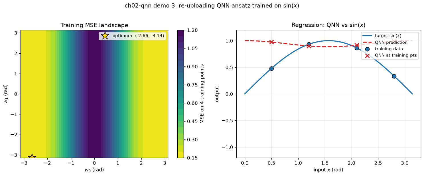
可视化：双图：MSE 等高线+拟合曲线 —— 1-qubit re-uploading ansatz 网格搜索最优点

对应教程：第 2 章 量子神经网络 中相关小节 · 依赖安装：pip install "unified-quantum[visualization,simulation]"

实现要点

核心：1-qubit data re-uploading ansatz |ψ(x, w)⟩ = RY(x) · RZ(w0) · RY(x) · RZ(w1) · |0⟩ 预测 f(x, w) = ⟨ψ(x, w)|Z|ψ(x, w)⟩ 用 4 个训练点 (x_i, sin(x_i)) 在 w ∈ [-π, π]² 上做网格搜索， 找到使 MSE 最小的 (w0*, w1*)，然后在同一网格上画出预测曲线。

完整源码

demos/ch02-qnn/03_qnn_ansatz.py

"""
ch02-qnn demo 3: 2-qubit re-uploading ansatz + sin regression

对应教程：chenzhaoyun.com/quantum-tutorial/ch02-quantum-nn/quantum-neural-network.html
核心：1-qubit data re-uploading ansatz
       |ψ(x, w)⟩ =  RY(x) · RZ(w0) · RY(x) · RZ(w1) · |0⟩
       预测      f(x, w) = ⟨ψ(x, w)|Z|ψ(x, w)⟩
用 4 个训练点 (x_i, sin(x_i)) 在 w ∈ [-π, π]² 上做网格搜索，
找到使 MSE 最小的 (w0*, w1*)，然后在同一网格上画出预测曲线。

依赖：pip install unified-quantum[visualization]
运行：python demos/ch02-qnn/03_qnn_ansatz.py
"""
from __future__ import annotations

from pathlib import Path

import matplotlib
matplotlib.use("Agg")
import matplotlib.pyplot as plt
import numpy as np

from uniqc import Circuit, submit_task, wait_for_result

OUT = Path(__file__).parent

SHOTS = 2000


def expectation_z_single(theta: float, phi: float, x: float, shots: int = SHOTS) -> float:
    """对 1-qubit re-uploading 线路 U(x,w)|0⟩ 测 ⟨Z⟩。

    线路顺序（从 |0⟩ 开始）：RY(x) → RZ(w0) → RY(x) → RZ(w1)
    """
    c = Circuit()
    c.ry(0, float(x))
    c.rz(0, float(theta))
    c.ry(0, float(x))
    c.rz(0, float(phi))
    c.measure(0)
    r = wait_for_result(submit_task(c, backend="dummy:local:simulator", shots=shots))
    p = r.probabilities
    return float(p.get("0", 0.0) - p.get("1", 0.0))


# === 1. 训练数据 ===
train_x = np.array([0.5, 1.2, 2.1, 2.8])              # 4 个输入点
train_y = np.sin(train_x)                              # 目标函数值

# === 2. 在 (w0, w1) 网格上搜索最小 MSE ===
GRID = 14
w0_grid = np.linspace(-np.pi, np.pi, GRID)
w1_grid = np.linspace(-np.pi, np.pi, GRID)
mse_grid = np.full((GRID, GRID), np.nan)

print(f"ch02-qnn-demo-3: grid search over {GRID}x{GRID} = {GRID*GRID} ansatz params")
total_evals = 0
for i, w0 in enumerate(w0_grid):
    for j, w1 in enumerate(w1_grid):
        preds = np.array([expectation_z_single(w0, w1, x) for x in train_x])
        mse_grid[i, j] = float(np.mean((preds - train_y) ** 2))
        total_evals += 1
print(f"  total quantum evaluations during search: {total_evals * len(train_x)}")

i_best, j_best = np.unravel_index(int(np.nanargmin(mse_grid)), mse_grid.shape)
w0_star, w1_star = float(w0_grid[i_best]), float(w1_grid[j_best])
best_mse = float(mse_grid[i_best, j_best])

# === 3. 在密网格上画预测曲线 ===
x_plot = np.linspace(0.0, np.pi, 60)
y_target = np.sin(x_plot)
y_pred = np.array([expectation_z_single(w0_star, w1_star, x) for x in x_plot])
print(f"  best (w0*, w1*) = ({w0_star:+.3f}, {w1_star:+.3f})  →  train MSE = {best_mse:.4f}")

# 训练点的预测
y_train_pred = np.array([expectation_z_single(w0_star, w1_star, x) for x in train_x])

# === 4. 绘图：损失等高线 + 预测曲线对比 ===
fig, (ax1, ax2) = plt.subplots(1, 2, figsize=(12.5, 5.0))

# 左图：损失景观
W0, W1 = np.meshgrid(w0_grid, w1_grid, indexing="ij")
cs = ax1.contourf(W0, W1, mse_grid, levels=20, cmap="viridis_r")
ax1.plot(w0_star, w1_star, "*", color="#ffd700", ms=18, mec="black", mew=0.8,
         label=f"optimum  ({w0_star:+.2f}, {w1_star:+.2f})")
ax1.set_xlabel(r"$w_0$ (rad)")
ax1.set_ylabel(r"$w_1$ (rad)")
ax1.set_title("Training MSE landscape")
ax1.legend(loc="upper right", fontsize=9)
cbar = plt.colorbar(cs, ax=ax1)
cbar.set_label("MSE on 4 training points")

# 右图：预测曲线 vs 真实 sin
ax2.plot(x_plot, y_target, color="#1f77b4", lw=2.2, label=r"target $\sin(x)$")
ax2.plot(x_plot, y_pred, color="#d62728", lw=2.2, ls="--", label="QNN prediction")
ax2.scatter(train_x, train_y, s=70, color="#1f77b4", ec="black", zorder=5, label="training data")
ax2.scatter(train_x, y_train_pred, s=70, marker="x", color="#d62728", zorder=5, lw=2,
            label="QNN at training pts")
ax2.set_xlabel(r"input $x$ (rad)")
ax2.set_ylabel("output")
ax2.set_title("Regression: QNN vs $\\sin(x)$")
ax2.set_ylim(-1.2, 1.2)
ax2.grid(alpha=0.3)
ax2.legend(loc="upper right", fontsize=9)

plt.suptitle("ch02-qnn demo 3: re-uploading QNN ansatz trained on $\\sin(x)$", y=1.02)
plt.tight_layout()
out_path = OUT / "03_qnn_ansatz.png"
plt.savefig(out_path, dpi=120, bbox_inches="tight")
plt.close()

# === 5. stdout 关键统计 ===
print("ch02-qnn-demo-3: QNN regression on sin(x)")
print(f"  training samples: {len(train_x)}  (x in {train_x.tolist()})")
print(f"  best ansatz params: w0* = {w0_star:+.4f}, w1* = {w1_star:+.4f}")
print(f"  training MSE      : {best_mse:.4f}")
print(f"  train y true  : {train_y.tolist()}")
print(f"  train y pred  : {[f'{v:+.4f}' for v in y_train_pred]}")
print(f"  curve points  : {len(x_plot)}  (x in [0, π])")
print(f"  PNG -> {out_path}")

运行结果

运行方式

# 仓库根目录执行；输出 PNG 到 demos/ch02-qnn/03_qnn_ansatz.png，关键统计到 stdout
.venv/bin/python3 demos/ch02-qnn/03_qnn_ansatz.py

---

← 本章演示 · ↑ 代码演示总索引 · ⌂ 教程门户